How can we implement Logistic Regression?

This article was published as a part of the Data Science Blogathon

Introduction

In this article, we will be learning about how we can implement logistic regression by writing Python code. You must be wondering what is logistic regression and what is the theory behind it? What python packages are involved while implementing logistic regression? You must be coming up with many more questions but I will try to answer as many as questions possible. Well, you have chosen the right article. So let’s begin our journey for logistic regression.

Topics to be covered in this article:

1. Introduction to Logistic Regression
2. How can we implement it?
3. Train your dataset
4. Sigmoid function
5. Calculating probability and making predictions
6. Calculating the cost
7. Reducting the cost using Gradient Descent
8. Testing you model
9. Predicting the values

Introduction to logistic regression

Logistic regression is a supervised learning algorithm that is widely used by Data Scientists for classification purposes as well as for calculating probabilities.  This is a very useful and easy algorithm. So, if you are new to the world of data science, then you will definitely enjoy learning this algorithm.  This algorithm is used for classifying both binary and multiclass datasets. If you want to know this algorithm in-depth, then I would suggest you read my article on Logistic regression: https://www.analyticsvidhya.com/blog/2021/05/logistic-regression-supervised-learning-algorithm-for-classification

Now we proceed to see how this algorithm can be implemented.

How can we implement it?

This algorithm can be implemented in two ways. The first way is to write your own functions i.e. you code your own sigmoid function, cost function, gradient function, etc. instead of using some library. The second way is,  of course as I mentioned, to use the Scikit-Learn library. The Scikit-Learn library makes our life easier and pretty good. All functions are already built-in, you just need to call those functions by passing the required parameters into it. However, if you are learning logistic regression for the first time, then I would suggest you write your own code instead of using the sci-kit-learn library. It does not mean that the mentioned library is not useful, I only want to make you learn the core concepts of this algorithm.

Train your dataset

Before you start working on a project, it is important for us to visualize the dataset. Once we have visualized your dataset, then we will move to the major part of the project. After visualization, we will train our dataset. The training process includes calculating the probability and the cost, and then reduce the cost on the available dataset. The given dataset helps us to train our model so that accurate predictions could be made. Once the model is trained, we check our accuracy on the validation set (this is the part of the dataset, usually we use 80% of our dataset as a training set and the rest 20% as a validation set.) A validation set is required to measure the accuracy of our trained model i.e. how our model will behave when it is exposed to similar unseen data. We compare the results of a validation set with their actual labels mentioned in the dataset.

So let’s visualize our data.

First load the data from the CSV file.

loan= pd.read_csv("loan_test.csv")

Then, have a look at the dataset with the following command:

import pandas as pd

loan= pd.read_csv("loan_test.csv")
print(loan.head(10))

The above image is an output of some dataset that aims to predict loan eligibility.

Of course, I recommend everyone who is learning ML and want to pursue a career in Data Science to learn plotting graphs using the Matplotlib library. It is going to be useful. Trust me!

By plotting your data on a graph, we can visualize the importance as well as the distribution of a particular factor.

Now in the next section, we’ll learn to make predictions using the sigmoid function.

Making predictions and implementing sigmoid function

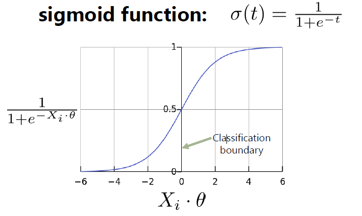
In logistic regression, we have to find the probability of each entry in the training set using the sigmoid function. The sigmoid function is a very important topic and must be clear to you if you have read my article (link given above.) So let me introduce a vector X and we will call it a ‘feature’ vector from now. Theta is a vector and we will call it the ‘weights’ vector. Look at the image below

(Image source: Google search)

Calculating probability and making predictions

Now you can clearly imagine what is sigmoid function from the above graph. The y-axis is the sigmoid function and the x-axis is the dot product of theta vector and X vector.

Now we’ll write a code for it:

def calc_sigmoid(z):
    p=1/(1+ np.exp(-z))
    p=np.minimum(p, 0.9999)
    p = np.maximum(p, 0.0001)
    return p

This is a sigmoid function that accepts a parameter z which is a dot product from the following function:

def calc_pred_func(theta,x):
    y=np.dot(theta,np.transpose(x))
    return calc_sigmoid(y)

The above function returns a probability value between [0,1].

Calculating the cost

Now the most important part is to reduce the cost of the predictions we made. So you must be wondering what is cost? It is the error in the calculations made from the existing labels. So we have to reduce our costs gradually. First, we calculate it using the given function:

def calc_error(y_pred, y_label):
    len_label=len(y_label)
    cost= (-y_label*np.log(y_pred) - (1-y_label)*np.log(1-y_pred)).sum()/len_label
    return cost

Now, we will work to reduce our cost using gradient descent

Reducing the cost using Gradient Descent

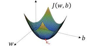
Just to tell you about the gradient descent, the graph looks like this for this technique:

Image source: google search

Now we will implement the gradient descent technique:

def gradient_descent(y_pred,y_label,x, learning_rate, theta):
    len_label=len(y_label)
    J= (-(np.dot(np.transpose(x),(y_label-y_pred)))/len_label)
    theta-= learning_rate*J
    #print("theta_0 shape: ",np.shape(theta),np.shape(J))
    return theta

Training Your Model:

def train(y_label,x, learning_rate, theta, iterations):
    list_cost=[]
    for i in range(iterations):
        y_pred=calc_pred_func(theta,x)
        theta=gradient_descent(y_pred,y_label,x, learning_rate, theta)
        if i%100==0:
            print("n iteration",i)
            print("y_label:",y_pred)
            print("theta:",theta)
        cost=calc_error(y_pred, y_label)
        list_cost.append(cost)
    print("final cost list: ",list_cost)
    return theta,list_cost,y_pred

We will call the train function to call all functions above and you’ll see the following graph when you plot costs per iterations:

We can see the graph declining i.e. the cost is reducing.

Testing your model

Now we will test our model on the validation set:

def classify(y_test):
    return np.around(y_test)

def predict(x_test,theta):

    y_test=np.dot(theta,np.transpose(x_test))

    #print(y_test)

    p=calc_sigmoid(y_test)

    print(p)

    return p

#for calculating accuracy based on validation set

'''

    Description of variables:

    x_test:numpy array (no. of rows in dataset, no. of features/columns)

    z_test: is added as column in x_test for the purpose of theta_0

    y_label_test: actual labels

    y_test= numpy array of probability (note: these are probabilities NOT classes)

    y_test_pred_labels= numpy array of classes based of probability (note: here it is classes NOT probability)

'''

x_test=loan.iloc[500:, 1:10].values

x_rows_test, x_columns_test= x_test.shape

z_test = np.ones((x_rows_test,1), dtype=float)

x_test=np.append(x_test,z_test,axis=1)

y_label_test=loan.loc[500:,"Status_New" ].values

y_label_test=y_label_test.astype(float)

x_test=x_test.astype(float)

y_test=predict(x_test,theta)

y_test_pred_labels=classify(y_test)

This will make a prediction on the validation set and you will get your output as the label 0 or 1.

I hope you enjoyed my article. This was all about its implementation.

About the Author:

Hi! I am Sarvagya Agrawal. I am pursuing B.Tech. from the Netaji Subhas University Of Technology. ML is my passion and feels proud to contribute to the community of ML learners through this platform. Feel free to contact me by visiting my website: sarvagyaagrawal.github.io

The media shown in this article are not owned by Analytics Vidhya and is used at the Author’s discretion.

Sarvagya

Hi, I'm Sarvagya Agrawal, Software Engineer, with a strong passion for utilizing technology to drive positive change in society. I believe that technology is not just a skill, but an art form that can be leveraged to transform the world.
My primary focus lies in machine learning and web development, with strong programming skills in Python. I have worked on innovative projects, including developing an AI model to calculate cardiovascular risk factors from OCTA scans using computer vision algorithms and creating an AI-based web application for calculating financial risk based on an individual's spending trends.