NumPy Library for Data Science

Introduction to NumPy Library:

A major part of Data Science is involved in Data Preprocessing and Data Cleaning which is tiresome and time-consuming. So that is where these modules of Python NumPy and Pandas prove handy in these processes. So these are used in different use cases based on the situation and required condition.

Let’s begin with NumPy without much delay:

NumPy (NP) is an acronym for Numerical Python as the name suggests, it is used for performing mathematical operations. Though we can use general mathematical operations, working on NP operations is much faster and has less time complexity compared to general ones and that is the main goal as we have tons and tons of data and we have to process faster.

Importing NumPy Library:

So that’s a basic overview of NP. Now let’s move on to practical implementation to understand what is said in words in the application.

This line of code is to be executed first before using NP functions. The code helps in importing the NP module so that we can use all the functions available inside the module. We have something called ‘as np’, which is used so that we can use just ‘np’ instead of writing ‘numpy’ everywhere in the code which helps to reduce the codes and our program would look simpler. At the core of NumPy is the ‘ndarray’, where nd stands for n-dimensional. This is similar to the list datatype but has slight differences.

This is how we create an NP array. This array contains elements of the same datatype but if it contains elements of other datatypes upper casting is done to convert all the elements to the same data type.

Creating a NumPy Array:

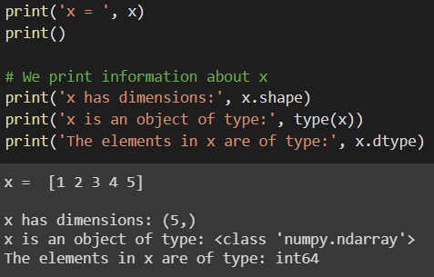
If we print ‘x’ it might look like a list as the elements are enclosed in square brackets. But if we try to print the details of variable ‘x’ we come to know that it has a dimension of 5, it is of the type NumPy array, and has a data type of ‘int64’ rather than the normal ‘int’ type.

shape -> It tells the dimension of the array, in our case it shows (5,) as there are only 5 elements and only 1 row.

type() -> This function can be used for any variable to determine the class it belongs to, in our case, it is of the class ‘numpy.ndarray’.

dtype -> As the name suggests this tells the data type of the variable, in our case since it belongs to class NumPy it is of the type – 64-bit integer.

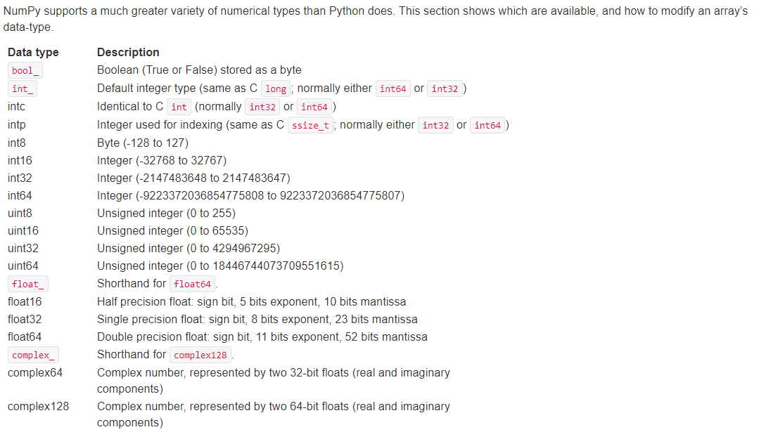
Please have a look at this image which clearly explains different data types. It is more clear to understand if we play with it and understand it.

Data Types available in NumPy:

2D- NumPy Array:

Till now we are dealing with the 1-D array. Let’s jump into a 2-D array. We can create a 2-D array by using the concept of a list of lists. Using this logic we can create a 2-D array.

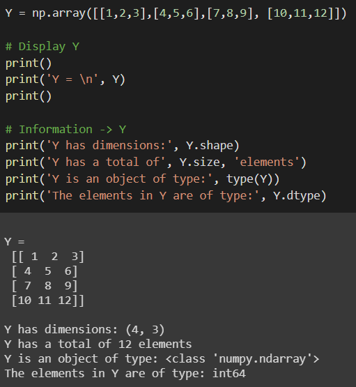
The above code shows how we create a 2-D array using the concept of using the concept list of lists. Then we print the details about the 2-D which is stored in variable Y. While we try to print the details of Y then we find that its dimensions are (4,3) which means it is a 2-D array. The remaining details are the same as the previous one.

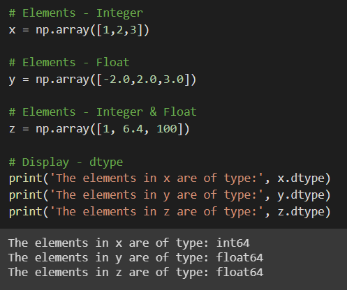
This shows script gives a clear understanding of how the type conversion is done while assigning data types using NumPy. The first and the second are assigned the same dtype as every other element in the array. Whereas the ultimate one i.e. variable ‘z’ has 2 elements of int64 type and the middle element is of float64 type. Though the total number of int64 type elements is more than float type elements the NumPy Array assigns it float64 type. This is called upcasting. Since all the elements of a NumPy Array must be of the same type, in this case, NumPy upcasts the integers in z to float to avoid losing precision in numerical computations.

Though NumPy Array automatically assigns the type we also have the option to assign the type as per our requirements. This can be understood by the following implementation.

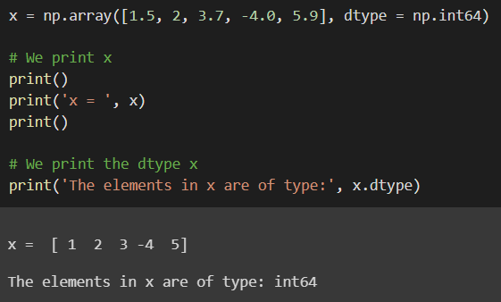
So though the elements given as input to the X are a combination of int64 and float64 type, as we have explicitly mentioned that the type must belong to int64. Hence, the elements are converted to the respective data types mentioned by the user.

Specialized NumPy Array:

With the help of the NumPy module, we can create many different types of arrays.

1. np.zeroes():

Let’s begin with the zeroes array. With the help of ‘np.zeroes()’ we can create an array full of zeroes according to the shape of the array.

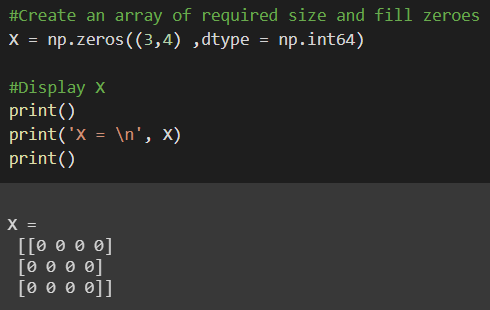
This picture gives the implementation of ‘np.zeroes()’ function. So we can mention the dimension of the according to the necessity.

2. np.ones():

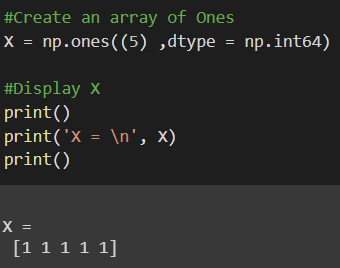
According to the previous array instead of zeroes we fill with 1’s using the ‘np.ones()’ function.

This image shows the implementation of the ‘np.ones()’ function.

3. np.eye():

This function is used to develop an array which is an Identity matrix of order n, where the matrix is square. This code gives an overview of the ‘np.eye()’ function.

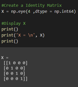
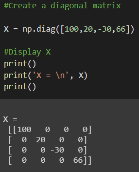
Instead of using eye() function if we use ‘np.diag()’ function we can generate a diagonal matrix where we can specify the diagonal elements.

Random Numpy Arrays:

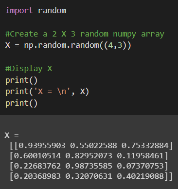
To implement this we first need to import the random function of the python, using the command “import random”. Then we use the random function of the random module to generate an array of the required order.

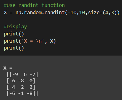
To further fine-tune the output we shall use the randint function of the random module to generate an array of the required order, within the specified range of integers.

This is the Link to Notebook for the readers as you can get benefitted from it as it not only has code implemented here but also has other extra functions described. Let’s get connected through LinkedIn. Also, refer to the NumPy Documentation for a better understanding of the NumPy library.

Sriniketh

A seasoned software and ML developer with likes to share knowledge on the latest skills, frameworks, and technologies. Writes about Data Science and Machine learning and love to build and ship projects.