This article was published as a part of the Data Science Blogathon
Introduction:
As we all know, Artificial Intelligence is being widely used around us – from reading the news on your mobile or analyzing that complex data at your workplace, AI has enhanced the speed, precision, and effectiveness of the human effort. The advancements in AI have helped us to achieve things that we thought were not possible before. Even having a pizza from your favorite restaurant at home is just a click away, thanks to AI.
Simply put, Artificial Intelligence stands for a computer or a computer program imitating human intelligence. It is accomplished by learning how the human brain thinks, learns, decides, and works while solving a problem. The outcomes of this study are then used as a basis for developing intelligent software and systems.
Get Personalized Learning Path! Set your goal and timeline. Get a path—under 2 mins.
There are 4 types of learning:
● Supervised learning.
● Unsupervised learning.
● Semi-supervised learning.
● Reinforced learning.
| Supervised | Unsupervised | Semi-supervised | Reinforced |
| Supervised learning is when the model is getting trained on a labelled dataset. | Unsupervised learning is when the model is getting trained on an unlabeled dataset, it is up to the algorithm to find underlying patterns in data. | It lays between supervised and unsupervised learning, in this, some learning data are labeled and others are not. | The algorithm evaluates its performance based on the feedback responses and reacts accordingly. |
This blog covers the supervised and unsupervised learning of AI, using Python and Iris dataset.
Table of contents:
- Introduction
- Iris dataset
- Supervised Learning
- Decision Tree
- Logistic Regression
- Unsupervised Learning
- K-means clustering
- Conclusion and References
Iris Dataset :
The data set contains 3 classes with 50 instances each, and 150 instances in total, where each class refers to a type of iris plant.
Class : Iris Setosa,Iris Versicolour, Iris Virginica
The format for the data: (sepal length, sepal width, petal length, petal width)

We will be training our models based on these parameters and further use them to predict the flower classes.
Understanding the data :
Download Iris dataset from https://www.kaggle.com/uciml/iris
Python Code:
import numpy as np
import pandas as pd
# import matplotlib.pyplot as plt
iris = pd.read_csv("Iris.csv") #Iris.csv is now a pandas dataframe
print("Head ==> \n",iris.head()) #prints first 5 values
print("Describe ==> \n",iris.describe())
#prints some basic statistical details like percentile,mean, std etc. of the data frame
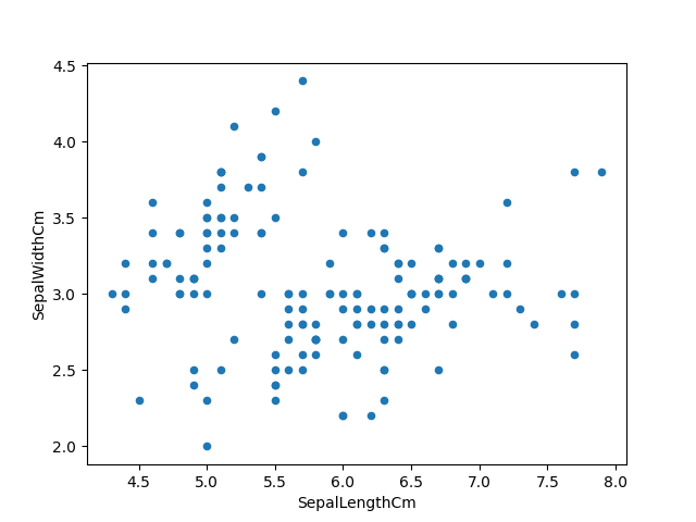
Visualizing the data using matplotlib :
iris.plot(kind="scatter", x="SepalLengthCm", y="SepalWidthCm") plt.show() |
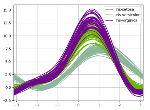
Visualizing the data using pandas’ andrew curves :
Andrews curves have the functional form:
f(t) = x_1/sqrt(2) + x_2 sin(t) + x_3 cos(t) +
x_4 sin(2t) + x_5 cos(2t) + …
Where x coefficients correspond to the values of each dimension and t is linearly spaced between -pi and +pi. Each row of the frame then corresponds to a single curve.
from pandas.plotting import andrews_curves
andrews_curves(iris.drop("Id", axis=1), "Species")
plt.show()
|
Preprocessing the dataset :
Using an inbuilt library called ‘train_test_split’, which divides our data set into a ratio of 80:20. 80% will be used for training, evaluating, and selection among our models and 20% will be held back as a validation dataset.
from sklearn.model_selection import train_test_split x = iris.iloc[:, :-1].values #last column values excluded y = iris.iloc[:, -1].values #last column value from sklearn.model_selection import train_test_split x_train,x_test,y_train,y_test = train_test_split(x,y,test_size=0.2,random_state=0) #Splitting the dataset into the Training set and Test set |
Supervised Learning :
Supervised machine learning algorithms are trained to find patterns using a dataset. The process is simple, It takes what has been learned in the past and then applies that to the new data. Supervised learning uses labelled examples to predict future patterns and events.
For example – when we teach a child that 2+2=4 or point them to the image of any animal to let them know what it is called.
Supervised learning is further divided into:
● Classification: Classification predicts the categorical class labels, which are discrete and unordered. It is a two-step process, consisting of a learning step and a classification step. There are various classification algorithms like – “Decision Tree Classifier”, “Random Forest”, “Naive Bayes classifier” etc.
● Regression: Regression is usually described as determining a relationship between two or more variables, like predicting the job of a person based on input data X.Some of the regression algorithms are: “Logistic Regression”, “Lasso Regression”, “Ridge Regression” etc.
Decision Tree Classifier:
The general motive of using a Decision Tree is to create a training model which can be used to predict the class or value of target variables by learning decision rules inferred from prior data(training data).
It tries to solve the problem, by using tree representation. Each internal node of the tree corresponds to an attribute, and each leaf node corresponds to a class label.
Using decision tree on Iris dataset :
from sklearn.tree import   DecisionTreeClassifier
from sklearn.metrics import accuracy_score
classifier = DecisionTreeClassifier() classifier.fit(x_train, y_train) #training the classifier y_pred = classifier.predict(x_test) #making precdictions print(classification_report(y_test, y_pred)) #Summary of the predictions made by the classifier print(confusion_matrix(y_test, y_pred)) #to evaluate the quality of the output print('accuracy is',accuracy_score(y_pred,y_test)) #Accuracy score
|
Precision – Accuracy of positive predictions.
Recall – Fraction of positives that were correctly identified.
F1 score – What percent of positive predictions were correct?
macro avg – averaging the unweighted mean per label
weighted avg – averaging the support-weighted mean per label
Heatmap for confusion matrix :
import seaborn as sns cm = confusion_matrix(y_test, y_pred) #Transform to df cm_df = pd.DataFrame(cm,index = ['setosa','versicolor','virginica'], columns = ['setosa','versicolor','virginica']) plt.figure(figsize=(5.5,4)) sns.heatmap(cm_df, annot=True) plt.ylabel('True label')
plt.xlabel('Predicted label')
plt.show() |
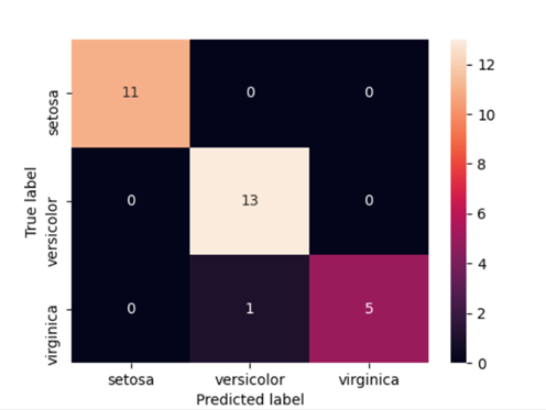
An insight we can get from the matrix is that the model was very accurate at classifying Setosa and Virginica (True Positive/All = 1.0). However, accuracy for Versicolor was lower(13/14=0.928).
Unsupervised Learning:
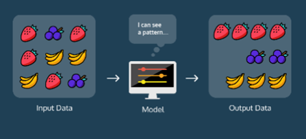
Unsupervised learning is used against data without any historical labels. The system is not subjected to a pre-determined set of outputs, correlations between inputs and outputs or a “correct answer.” The algorithm must figure out what it is viewing by itself, as it does not have any storage of reference points. The goal is to explore the data and find some sort of patterns or structures.
Unsupervised learning can be classified into:
● Clustering: Clustering is the task of dividing the population or data points into several groups, such that data points in a group are homogenous to each other than those in different groups. There are numerous clustering algorithms, some of them are – “K-means clustering algorithms”, “mean shift”, “hierarchal clustering”, etc.
● Association: An association rule is an unsupervised learning method that is used for finding the relationships between variables in a large database. It determines the set of items that occurs together in the dataset.
K-means Clustering:
The goal of the K-means clustering algorithm is to find groups in the data, with the number of groups represented by the variable K. The algorithm works iteratively to assign each data point to one of the K groups based on the features that are provided.
The outputs of executing a K-means on a dataset are:
● K centroids: Centroids for each of the K clusters identified from the dataset.
● Labels for the training data: Complete dataset labelled to ensure each data point is assigned to one of the clusters.
Using K-means clustering on Iris dataset:
from sklearn.datasets import load_iris
from sklearn.cluster import KMeans
iris_data=load_iris() #loading iris dataset from sklearn.datasets iris_df = pd.DataFrame(iris_data.data, columns = iris_data.feature_names) #creating dataframe kmeans = KMeans(n_clusters=3,init = 'k-means++', max_iter = 100, n_init = 10, random_state = 0) #Applying Kmeans classifier y_kmeans = kmeans.fit_predict(x) print(kmeans.cluster_centers_) #display cluster centers plt.scatter(x[y_kmeans == 0, 0], x[y_kmeans == 0, 1],s = 100, c = 'red', label = 'Iris-setosa') plt.scatter(x[y_kmeans == 1, 0], x[y_kmeans == 1, 1],s = 100, c = 'blue', label = 'Iris-versicolour') plt.scatter(x[y_kmeans == 2, 0], x[y_kmeans == 2, 1],s = 100, c = 'green', label = 'Iris-virginica') #Visualising the clusters - On the first two columns plt.scatter(kmeans.cluster_centers_[:, 0], kmeans.cluster_centers_[:,1],s = 100, c = 'black', label = 'Centroids') #plotting the centroids of the clusters plt.legend() plt.show() |
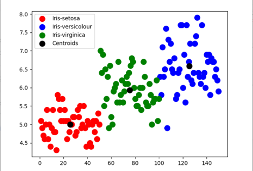
An insight we can get from the scatterplot is the model’s accuracy in determining Setosa and Virginica is comparatively more to Versicolour.
Conclusion :
We have explored and preprocessed the Iris dataset using the sklearn. dataset as well as using the Iris.csv file. Also, learned about supervised and unsupervised learning and implemented the Decision tree algorithm and K-means clustering algorithm.
References:
About the Author:
Hey there reader, I am Yashi Saxena, currently working in TCS as a System Engineer. AI, ML and NLP have always been my interest, so here I am making an effort to learn more about this field. You can connect with me on Linkedin: https://www.linkedin.com/in/yashi-saxena-7a9522194/


Fantastic article Yashi. Keep up the good work👍
Was really helpful. Thanks