This article was published as a part of the Data Science Blogathon
Introduction:
In this blog, we will discuss the classification of music files based on the genres. Generally, people carry their favorite songs on smartphones. Songs can be of various genres. With the help of deep learning techniques, we can provide a classified list of songs to the smartphone user. We will apply deep learning algorithms to create models, which can classify audio files into various genres. After training the model, we will also analyze the performance of our trained model.
Dataset:
We will use GITZAN dataset, which contains 1000 music files. Dataset has ten types of genres with uniform distribution. Dataset has the following genres: blues, classical, country, disco, hiphop, jazz, reggae, rock, metal, and pop. Each music file is 30 seconds long.
Process Flow:
Figure 01 represents the overview of our methodology for the genre classification task. We will discuss each phase in detail. We train three types of deep learning models to explore and gain insights from the data.
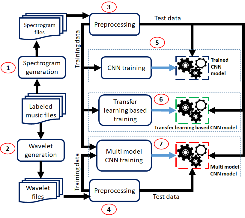
First, we need to convert the audio signals into a deep learning model compatible format. We use two types of formats, which are as follows:
1. Spectrogram generation:
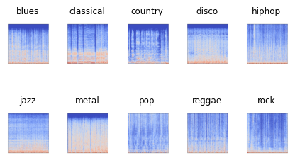
A spectrogram is a visual representation of the spectrum signal frequencies as it varies with time. We use librosa library to transform each audio file into a spectrogram. Figure 02 shows spectrogram images for each type of music genre.
2. Wavelet generation: –
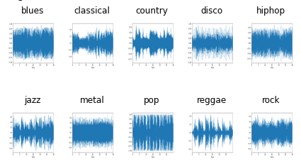
The Wavelet Transform is a transformation that can be used to analyze the spectral and temporal properties of non-stationary signals like audio. We use librosa library to generate wavelets of each audio file. Figure 03 shows wavelets of each type of music genre.
3, 4. Spectrogram and Wavelet preprocessing
From Figure 02 and 03, it is clear that we treat our data as image data. After generating spectrograms and wavelets, we apply general image preprocessing steps to generate training and testing data. Each image is of size (256, 256, 3).
5. Basic CNN model training:
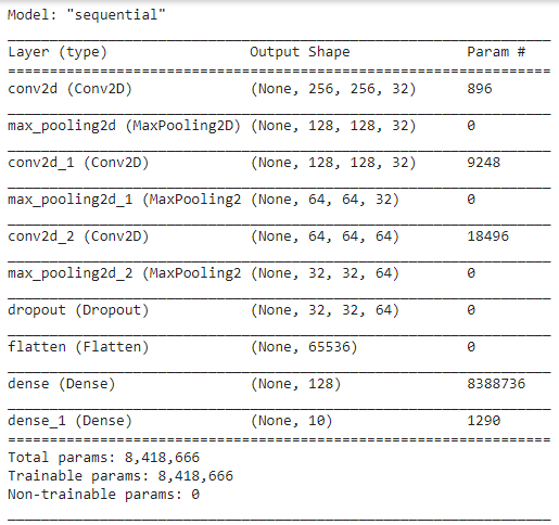
After preprocessing the data, we create our first deep learning model. We construct a Convolution Neural Network model with required input and out units. The final architecture of our CNN model is shown in Figure 04. We use only spectrogram data for the training and testing.
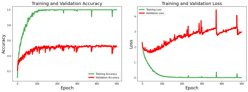
We train our CNN model for 500 epochs with Adam optimizer at a learning rate of 0.0001. We use categorical cross-entropy as the loss function. Figure 05 shows the training and validation losses and model performance in terms of accuracy.
6. Transfer learning-based model training
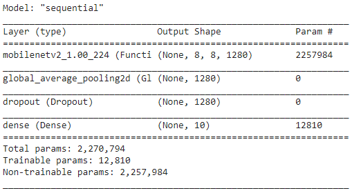
We have only 60 samples of each genre for training. In this case, transfer learning could be a useful option to improve the performance of our CNN model. Now, we use the pre-trained mobilenet model to train the CNN model. A schematic architecture is shown in Figure 06.
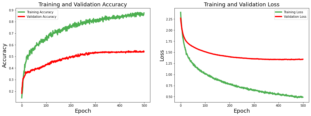
The transfer learning-based model is trained with the same settings as used in the previous model. Figure 07 shows the training and validation loss and model performance in terms of accuracy. Here, also we use only spectrogram data for the training and testing.
7. Multimodal training
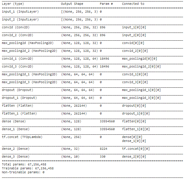
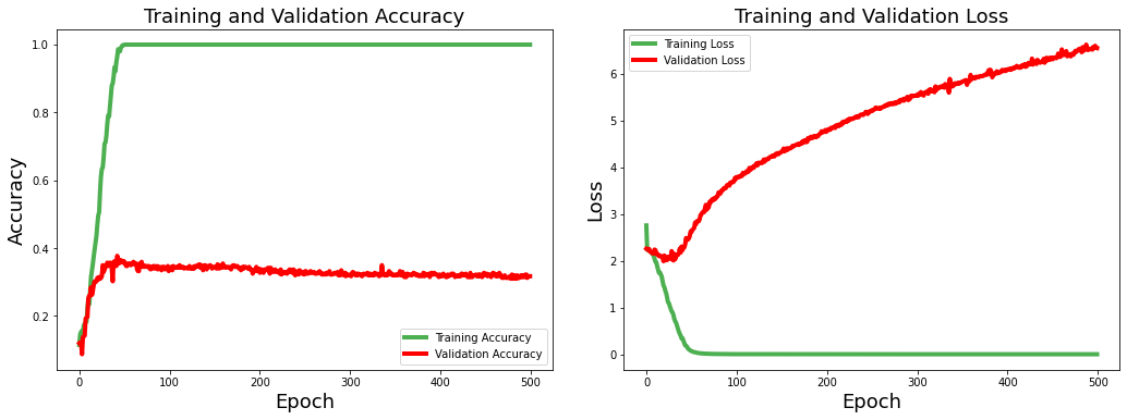
We will pass both spectrogram and wavelet data into the CNN model for the training in this experiment. We are using the late-fusion technique in this multi-modal training. Figure 08 represents the architecture of our multi-modal CNN model. Figure 09 shows the loss and performance scores of the model with respect to epochs.
Comparison:
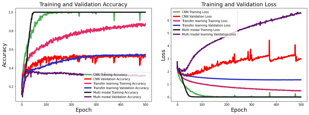
Figure 10 shows a comparative analysis of the loss and performance of all three models. If we analyze the training behavior of all three models, we found that the basic CNN model has large fluctuations in its loss values and performance scores for training and testing data. The multimodal model has shown the least variance in performance. Transfer learning model performance increases gradually compared to multimodal and basic CNN models. Validation loss value shot up suddenly after the 30 epochs. On the other side, validation loss decreases continuously for the other two models.
Testing the models
After training our models, we test each model on the 40% test data. We calculate precision, recall, and F-score for each music genre (class). Our dataset is balanced; therefore, the macro average and weighted average of precision, recall, and F-score are the same.
1. Basic CNN model
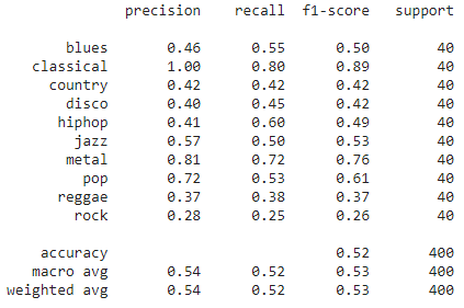
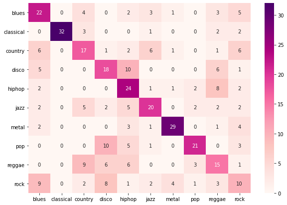
Figure 11 presents the results of our CNN model on the test data. CNN model was able to classify “classical” genre music with the highest F1-score. CNN performed worst for “Rock” and “reggae” genre music. Figure 12 shows the confusion matrix of the CNN model on the test data.
2. Transfer learning based model
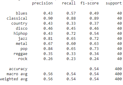
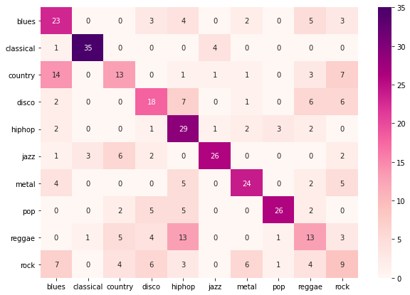
We used the transfer learning technique to improve the performance of genre classification. Figure 13 presents the results of the transfer learning-based model on test data. F1-score for “hiphop”, “jazz”, and “pop” genres increased due to transfer learning. If we look at overall results, we have achieved only a minor improvement after applying transfer learning. Figure 14 shows the confusion matrix for the transfer learning model on the test data.
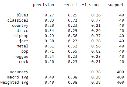
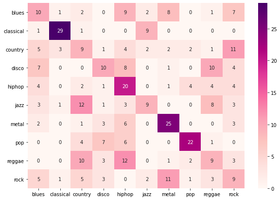
3. Multimodal-based model: We have used both spectrogram and wavelet data to train the multimodal-based model. In the same way, we perform the testing. We have found very surprising results. Instead of improvement, our performance reduced drastically. We have achieved only 38% of F1-score while using a multi-modal approach. Figure 16 shows the confusion matrix of the multimodal-based model on the test data.
Conclusion:
In this post, we have performed music genre classification using Deep learning techniques. The transfer learning-based model has performed best among all three models. We have used the Keras framework for the implementation on the google Collaboratory platform. Source code is available at the following GitHub link along with spectrogram and wavelet data on google drive. You don’t need to generate spectrograms and wavelets from the audio files.
GitHub Link. . Spectrogram and wavelets data link.
The media shown in this article are not owned by Analytics Vidhya and are used at the Author’s discretion.


