This article was published as a part of the Data Science Blogathon
Introduction
This article is part of an ongoing blog series on Natural Language Processing (NLP). In the previous article, we discussed all the basic concepts related to Topic modelling. Now, from this article, we will start our journey towards learning the different techniques to implement Topic modelling. In this article, we will be discussing a very basic technique of topic modelling named Non-negative Matrix Factorization (NMF).
So, In this article, we will deep dive into the concepts of NMF and also discuss the mathematics behind this technique in a detailed manner.
This is part-15 of the blog series on the Step by Step Guide to Natural Language Processing.
Table of Contents
1. What is Non-negative Matrix Factorization (NMF)?
2. General Case of NMF
3. Maths Behind NMF
4. Objective Function in NMF
5. Some heuristics to initialize the matrix W and H
6. NMF in Action or real-life example
7. Projects to accelerate your NLP Journey
Non-Negative Matrix Factorization (NMF)
Non-Negative Matrix Factorization is a statistical method that helps us to reduce the dimension of the input corpora or corpora. Internally, it uses the factor analysis method to give comparatively less weightage to the words that are having less coherence.
Some Important points about NMF:
1. It belongs to the family of linear algebra algorithms that are used to identify the latent or hidden structure present in the data.
2. It is represented as a non-negative matrix.
3. It can also be applied for topic modelling, where the input is the term-document matrix, typically TF-IDF normalized.
- Input: Term-Document matrix, number of topics.
- Output: Gives two non-negative matrices of the original n-words by k topics and those same k topics by the m original documents.
- In simple words, we are using linear algebra for topic modelling.
4. NMF has become so popular because of its ability to automatically extract sparse and easily interpretable factors.
Below is the pictorial representation of the above technique:
Image Source: Google Images
As described in the image above, we have the term-document matrix (A) which we decompose it into two the following two matrices,
- First matrix: It has every topic and what terms in it,
- Second matrix: It has every document and what topics in it.
For Example,

Image Source: Google Images
General case of NMF
Let’s have an input matrix V of shape m x n. This method of topic modelling factorizes the matrix V into two matrices W and H, such that the shapes of the matrix W and H are m x k and k x n respectively.
In this method, the interpretation of different matrices are as follows:
- V matrix: It represents the term-document matrix,
- H matrix: Each row of matrix H is a word embedding,
- W matrix: Each column of the matrix W represents the weightage of each word gets in each sentence i.e, semantic relation of words with each sentence.
But the main assumption that we have to keep in mind is that all the elements of the matrices W and H are positive given that all the entries of V are positive.
Image Source: Google Images
Let’s try to look at the practical application of NMF with an example described below:
Imagine we have a dataset consisting of reviews of superhero movies.
Input matrix: Here in this example, In the document term matrix we have individual documents along the rows of the matrix and each unique term along with the columns.
In case, the review consists of texts like Tony Stark, Ironman, Mark 42 among others. It may be grouped under the topic Ironman. In this method, each of the individual words in the document term matrix is taken into consideration.
While factorizing, each of the words is given a weightage based on the semantic relationship between the words. But the one with the highest weight is considered as the topic for a set of words. So this process is a weighted sum of different words present in the documents.
Maths behind NMF
As we discussed earlier, NMF is a kind of unsupervised machine learning technique. The main goal of unsupervised learning is to quantify the distance between the elements. To measure the distance, we have several methods but here in this blog post we will discuss the following two popular methods used by Machine Learning Practitioners:
- Generalized Kullback–Leibler divergence
- Frobenius norm
Let’s discuss each of them one by one in a detailed manner:
Generalized Kullback–Leibler Divergence
It is a statistical measure that is used to quantify how one distribution is different from another. As the value of the Kullback–Leibler divergence approaches zero, then the closeness of the corresponding words increases, or in other words, the value of divergence is less.
The formula for calculating the divergence is given by:
Below is the implementation of Frobenius Norm in Python using Numpy:

Now, let’s try the same thing using an inbuilt library named Scipy of Python:

Frobenius Norm
It is another method of performing NMF. It is defined by the square root of the sum of absolute squares of its elements. It is also known as the euclidean norm. The formula for calculating the Frobenius Norm is given by:
Below is the implementation of Frobenius Norm in Python using Numpy:

It is considered a popular way of measuring how good the approximation actually is. Or if you want to find the optimal approximation to the Frobenius norm, you can compute it with the help of truncated Singular Value Decomposition (SVD).
Test Your Previous Knowledge
1. How many trigrams are possible for the given sentence?
"Despite past associations with left wing organizations Oppenheimer welcomed the opportunity to play a part in the war effort"
- 15
- 17
- 19
- None of these
2. Consider the following corpus of 4 sentences. Find the total count of unique bi-grams for which the likelihood will be estimated. (Assume we do not perform any pre-processing)
today is Nayan's birthday
she loves ice cream
she is also fond of cream cakes
we will celebrate her birthday with ice cream cake
- 20
- 23
- 27
- None of these
3. Find out the output of the following program:
import re
re.sub('technology', 'limited', 'Wipro technology')
- Wipro
- limited
- Wipro limited
- Wipro technology
Objective Function in NMF
Given the original matrix A, we have to obtain two matrices W and H, such that
A= WH
NMF has an inherent clustering property, such that W and H described the following information about the matrix A:
- A (Document-word matrix): Input that contains which words appear in which documents.
- W (Basis vectors): The topics (clusters) discovered from the documents.
- H (Coefficient matrix): The membership weights for the topics in each document.
Based on our prior knowledge of Machine and Deep learning, we can say that to improve the model and want to achieve high accuracy, we have an optimization process. There are two types of optimization algorithms present along with the scikit-learn package.
- Coordinate Descent Solver
- Multiplicative update Solver
In this technique, we can calculate matrices W and H by optimizing over an objective function (like the EM algorithm), and updates both the matrices W and H iteratively until convergence.
What exactly happens in this objective function?
In this objective function, we try to measure the error of reconstruction between the matrix A and the product of its factors W and H, on the basis of Euclidean distance.
Now, by using the objective function, our update rules for W and H can be derived, and we get:
For updation of elements of Matrix W:
For updation of elements of Matrix H:
Here we parallelly update the values and using the new matrices that we get after updation W and H, we again compute the reconstruction error and repeat this process until we converge.
So, as a concluding step we can say that this technique will modify the initial values of W and H up to the product of these matrices approaches to A or until either the approximation error converges or the maximum iterations are reached.
In our case, the high-dimensional vectors or initialized weights in the matrices are going to be TF-IDF weights but it can be really anything including word vectors or a simple raw count of the words. But there are some heuristics to initialize these matrices with the goal of rapid convergence or achieving a good solution. Now, in the next section let’s discuss those heuristics.
Some heuristics to initialize the matrix W and H
You can initialize W and H matrices randomly or use any method which we discussed in the last lines of the above section, but the following alternate heuristics are also used that are designed to return better initial estimates with the aim of converging more rapidly to a good solution.
1. Use some clustering method, and make the cluster means of the top r clusters as the columns of W, and H as a scaling of the cluster indicator matrix (which elements belong to which cluster).
2. Finding the best rank-r approximation of A using SVD and using this to initialize W and H.
3. Picking r columns of A and just using those as the initial values for W.
Real-life Application of NMF
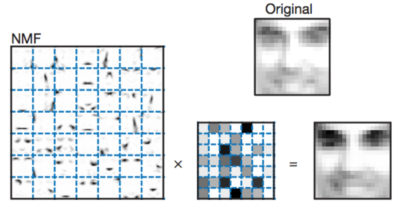
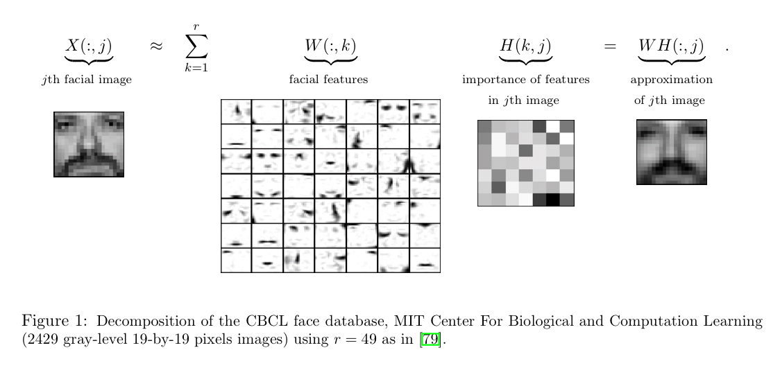
Image Processing uses the NMF. Let’s look at more details about this.
Say we have a gray-scale image of a face containing p number of pixels and squash the data into a single vector such that the ith entry represents the value of the ith pixel. Let the rows of X ∈ R(p x n) represent the p pixels, and the n columns each represent one image.
Now, in this application by using the NMF we will produce two matrices W and H. Now, a question may come to mind:
What exactly these matrices represent related to the given Use-Case?
Matrix W: The columns of W can be described as images or the basis images.
Matrix H: This matrix tells us how to sum up the basis images in order to reconstruct an approximation to a given face.

Image Source: Google Images
In the case of facial images, the basis images can be the following features:
- Eyes,
- Noses,
- Mustaches,
- Lips,
And the columns of H represents which feature is present in which image.
NOTE: After reading this article, now it’s time to do NLP Project. So, In the next section, I will give some projects related to NLP. Please try to solve those problems by keeping in mind the overall NLP Pipeline.
Projects to accelerate your NLP Journey
Now, it’s time to take the plunge and actually play with some real-life datasets so that you have a better understanding of all the concepts which you learn from this series of blogs. So are you ready to work on the challenge? So, without wasting time, now accelerate your NLP journey with the following Practice Problems:
Identify the sentiment of tweets
Practice Problem: Identify the Sentiments
To detect hate speech in tweets
Practice Problem: Twitter Sentiment Analysis
This ends our Part-15 of the Blog Series on Natural Language Processing!
Other Blog Posts by Me
You can also check my previous blog posts.
Previous Data Science Blog posts.
Here is my Linkedin profile in case you want to connect with me. I’ll be happy to be connected with you.
For any queries, you can mail me on [email protected]
End Notes
Thanks for reading!
I hope that you have enjoyed the article. If you like it, share it with your friends also. Something not mentioned or want to share your thoughts? Feel free to comment below And I’ll get back to you. 😉


