12 Matrix Operations You Should Know While Starting your Deep Learning Journey

This article was published as a part of the Data Science Blogathon

Introduction

If you start to learn deep learning, the first thing you will be exposed to is the concepts of Linear Algebra which give you better intuition on how algorithms really work under the hood, which enables you to make better decisions. In Deep Learning, a feed-forward neural network is a most simple and highly useful network. Under the hood, the feed-forward neural network is just a composite function, that multiplies some matrices and vectors together.

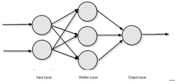
Image Source: Link

It is not that vectors and matrices are the only way to do these operations but they become highly efficient if you do so. The core data structures behind Deep-Learning includes

• Scalars,
• Vectors,
• Matrices, and
• Tensors.

Matrix operations are used in the description of many Deep learning algorithms.

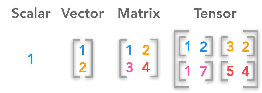
Image Source: Link

So if you really want to be a professional in the field of Deep Learning, then you cannot escape mastering some of these concepts. So, In this article, we will discuss important linear algebra matrix operations that are used in the description of deep learning methods.

Table of Contents

The topics which we will be discussing in this article are as follows:

• What are Matrices?
• How to add and subtract different matrices?
• How to find the shape and size of a given matrix?
• How to convert a dense matrix to a sparse matrix?
• How to find the transpose of a matrix?
• How to find the mean, variance, and standard deviation of a matrix?
• How to find the trace of a matrix?
• How to extract the minimum and maximum elements from a matrix?
• How to find the determinant of a matrix?
• How to multiply the given matrices?
• How to apply the particular operation to each element of a matrix?
• How to find the inverse of a matrix?
• How to reshape the matrix to a different size?

What are Matrices?

Matrices are rectangular arrays consisting of numbers and can be seen as 2nd-order tensors. If m and n are positive integers, that is m, n ∈ ℕ then the m×n matrix contains m*n numbers of elements, with m number of rows and n number of columns.

The pictorial representation of an m×n matrix is shown below:

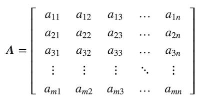
Image Source: Link

Sometimes, instead of describing the full matrix components, we use the following abbreviation of a matrix:

For Example-

In this example, with the help of the numpy library, we will create a matrix. And also check the dimension of the formed matrix.

import numpy as np
matrix = np.array([[45,34],[67,58]])
# Create a matrix
print("The original matrix is given by n", matrix)
# Check the dimension of the matrix
print("The dimension of the given matrix is", matrix.ndim)

Matrices Addition and Subtraction

Image Source: Link

In this section, we will be doing matrices addition and subtraction using the methods add and subtract. These methods take two arguments and return the sum and difference of those matrices respectively. If the shape of the matrices is not the same it throws an error saying, the addition or subtraction not possible.

matrix_1 = np.array([[45,34],[67,58]])
matrix_2 = np.array([[35,24],[57,48]])
# Add the two matrices
print("The result after adding matrix 1 and matrix 2 is given by n" , np.add(matrix_1, matrix_2))
# Subtract one matrix from the other matrices
print("The result after subtracting matrix 1 from matrix 2 is given by n" , np.subtract(matrix_1, matrix_2))
print("The result after subtracting matrix 2 from matrix 1 is given by n" , np.subtract(matrix_2, matrix_1))

Output:

The result after adding matrix 1 and matrix 2 is given by 
 [[ 80  58]
 [124 106]]
The result after subtracting matrix 1 from matrix 2 is given by 
 [[10 10]
 [10 10]]
The result after subtracting matrix 2 from matrix 1 is given by 
 [[-10 -10]
 [-10 -10]]

Shape and Size of a Matrix

 In this section, we will be finding shape i.e, the number of rows and columns in the given matrix and size i.e, number of elements in the matrix of a given matrix.

matrix = np.array([[45,34,75],[67,58,89]])
# Finding number of rows and columns in the matrix
print("The number of rows and columns in the given matrix are " + str(matrix.shape[0]) + " and " + str(matrix.shape[1]) + " respectively")
# Number of elements in the matrix
print("The size of the given matrix is" , matrix.size)

Output:

The number of rows and columns in the given matrix are 2 and 3 respectively
The size of the given matrix is 6

Converting a given Dense matrix to a Sparse Matrix

Let’s first understand what exactly it means by Sparse and Dense Matrix.

A sparse matrix is a matrix that consists of mostly zero values. And Sparse matrices are different from matrices with mostly non-zero values, which are Known as dense matrices.

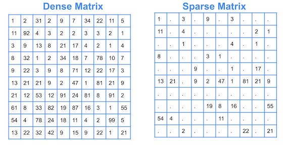
                                                       Image Source: Link

from scipy import sparse
# Create a Dense Matrix
dense_matrix = np.array([[0,0],[0,17],[78,0]])
# Convert Dense matrix to Sparse matrix
sparse_matrix = sparse.csr_matrix(dense_matrix)
print("The sparse matrix corresponding to a given dense matrix is given by n" , sparse_matrix)

Output:

The sparse matrix corresponding to a given dense matrix is given by 
   (1, 1)	17
  (2, 0)	78

Matrix Transpose

In Matrix Transpose, we can convert a row vector to a column vector and vice versa i.e, row becomes columns and columns becomes rows.

If we have matrix A = [aij]_mxn, then the transpose of this matrix is A^T = [aji]_n×m

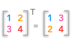
Image Source: Link  

import numpy as np
matrix = np.array([[45,34],[67,58]])
print("The original matrix is given by n" , matrix)
print("The transpose matrix of the given matrix is n" , matrix.T)

Output:

The original matrix is given by 
 [[45 34]
 [67 58]]
The transpose matrix of the given matrix is 
 [[45 67]
 [34 58]]

Mean, Variance, and Standard Deviation of a Matrix

In this section, we will try to find some statistical things related to a matrix. Here we calculate the mean, variance, and standard deviation of the matrix using the numpy functions.

import numpy as np
matrix = np.array([[45,34],[67,58], [23,89]])
# Finding the mean of a matrix elements
print("The mean of the elements of a matrix is equal to", np.mean(matrix))
# Finding the Variance of a matrix elements
print("The variance of the elements of a matrix is equal to", np.var(matrix))
# Finding the Standard Deviation of a matrix elements
print("The standard deviation of the elements of a matrix is equal to", np.std(matrix))
print("The standard deviation of the elements of a matrix is equal to", np.sqrt(np.var(matrix)))

Output:

The mean of the elements of a matrix is equal to 52.666666666666664
The variance of the elements of a matrix is equal to 473.5555555555555
The standard deviation of the elements of a matrix is equal to 21.761331658599286
The standard deviation of the elements of a matrix is equal to 21.761331658599286

Trace of a Matrix

                                                    Image Source: Link

In this section, we will try to find the trace of a matrix i.e, the sum of all the diagonal elements present in a given matrix.

import numpy as np
matrix = np.array([[1,2,3],[4,5,6], [7,8,9]])
# Get the diagonal elements of a matrix
print("The diagonal elements of a given matrix are n", matrix.diagonal())
# Finding the trace of the matrix
print("The trace of a given matrix is equal to", matrix.diagonal().sum())

Output:

The diagonal elements of a given matrix are 
 [1 5 9]
The trace of a given matrix is equal to 15

Finding minimum and maximum elements from a Matrix

In this section, we will try to find the minimum and maximum elements of a matrix i.e, the element with the highest and lowest value among all the elements.

import numpy as np
matrix = np.array([[1,2,3],[4,5,6], [7,8,9]])
# Find the minimum element of the matrix
print("The minimum element in a given matrix is", np.min(matrix))
# Find the maximum element of the matrix
print("The maximum element in a given matrix is", np.max(matrix))

Output:

The minimum element in a given matrix is 1
The maximum element in a given matrix is 9

Determinant of a Matrix

                                                            Image Source: Link

In this section, we will try to find the determinant of a matrix. Here to calculate the determinant, we use the linear algebra module present in the Numpy package.

import numpy as np
matrix = np.array([[1,2,4],[3,4,6], [7,8,5]])
# Find the determinant of the matrix
print("The determinant of the given matrix is equal to", np.linalg.det(matrix))

Output:

The determinant of the given matrix is equal to 9.999999999999993

Matrix Multiplication

A matrix of shape (m x n) and B matrix of shape (n x p) multiplied gives C of shape (m x p). Remember while multiplying the matrices is that the number of columns in the first matrix is the same as the number of rows in the second matrix to perform multiplication without error.

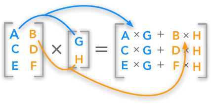
                                                      Image Source: Link

In this section, we will try to find the multiplication of two matrices.

import numpy as np
matrix_1 = np.array([[45,34],[67,58]])
matrix_2 = np.array([[35,24],[57,48]])
print("The matrix multiplication of given two matrices is given by n", np.matmul(matrix_1, matrix_2))

Output:

The matrix multiplication of given two matrices is given by 
 [[3513 2712]
 [5651 4392]]

Element wise operations using an inline function (Lambda)

In this example, we will try to add a certain value to each of the elements of a matrix.

import numpy as np
matrix = np.array([[1,2,4],[3,4,6], [7,8,5]])
addition = lambda i:i+5
add_5_vec = np.vectorize(addition)
print("The matrix after adding 5 to all its elements is n", add_5_vec(matrix))

Output:

The matrix after adding 5 to all its elements is 
 [[ 6  7  9]
 [ 8  9 11]
 [12 13 10]]

Inverse of a Matrix

In this section, we will try to find the inverse of a matrix.

import numpy as np
matrix = np.array([[1,2,4],[3,4,6], [7,8,5]])
# Finding the inverse of a matrix
print("The inverse matrix of a given matrix is n", np.linalg.inv(matrix))

Output:

The inverse matrix of a given matrix is 
 [[-2.8  2.2 -0.4]
 [ 2.7 -2.3  0.6]
 [-0.4  0.6 -0.2]]

Reshape a given Matrix

In this section, we will try to reshape a given matrix i.e, change the shape of the given matrix. But here we have to note that the size remains constant after reshaping the matrix i.e,  the number of elements remains the same.

import numpy as np
matrix = np.array([[1,2,4],[3,4,6],[7,8,5],[9,2,1]])
print("The reshaped matrix is given by n", matrix.reshape(6,2))

Output:

The reshaped matrix is given by 
 [[1 2]
 [4 3]
 [4 6]
 [7 8]
 [5 9]
 [2 1]]

Other Blog Posts by Me

You can also check my previous blog posts.

Previous Data Science Blog posts.

LinkedIn

Here is my Linkedin profile in case you want to connect with me. I’ll be happy to be connected with you.

Email

For any queries, you can mail me on [email protected]

End Notes

Thanks for reading!

I hope that you have enjoyed the article. If you like it, share it with your friends also. Something not mentioned or want to share your thoughts? Feel free to comment below And I’ll get back to you. 😉

Chirag Goyal

I am a B.Tech. student (Computer Science major) currently in the pre-final year of my undergrad. My interest lies in the field of Data Science and Machine Learning. I have been pursuing this interest and am eager to work more in these directions. I feel proud to share that I am one of the best students in my class who has a desire to learn many new things in my field.