This article was published as a part of the Data Science Blogathon
Introduction
Ever since history, people have always been interested in forecasting, be it a person’s future or a nation’s. From the play, Julius Caesar to the historic novel Ponniyin Selvan, the forecasters play a very important role. We are still curious about the predictions of the Mayan calendar, which Mayans created thousands of years ago.
All forecasting is predictions, but not all predictions are forecasting. There are so many prediction problems that involve a time component, which makes time series forecasting an important area in machine learning. Before we use a time series approach to a prediction problem, there are few things we must know about time-series forecasting. In this article, we will look at some of the must-know terms of time series forecasting.
Goals, Planning, and Forecasting
Forecasting is done in a lot of places for eg., weather prediction, stock market prediction, scheduling production, transportation, etc., The terms forecast, goals, and planning are often confused with each other and used interchangeably. But, they are not the same.
Goals: We know what goals are, it is what we expect to happen or what we want to happen. Say, you fix a goal to finish writing an essay in 4 hours.
Planning: Planning is dependent on the goal. It is determining the actions that are required to achieve your goal. It is breaking down your bigger goal into smaller things. Say, you finish researching your essay in 2 hours, write a draft and make some edits in 1 hour and write your final essay in 1 hour.
Forecasting: It is about predicting the future as accurately as possible when you have all the necessary information that might impact the forecasts such as historical data and knowledge of future events. Say, when you’ve written an essay already and you predict that you’ll be half done by the end of two hours.
So, what can I forecast and the period for which I can forecast? Based on the application, short-term, medium-term, and long-term forecasts can be used by the organization. Several approaches are to develop a forecasting system that is by an organization to predict uncertain events.
Types of forecasting based on time
Short-term forecasting: They are used in scheduling such as scheduling personnel, production, and transportation. Forecasts of demand are often required for short-term forecasting. Eg.: Buying groceries for a month.
Medium-term forecasting: When you are determining future resource requirements such as buying raw materials, hiring employees, or buying machinery or equipment, medium-term forecasting must be used. Eg.: When you are buying a phone, you would look if the features will stay relatively new for a while, not just for a month or 10 years.
Long-term forecasting: In strategic planning, we must consider market opportunities, environmental factors, and internal resources. Long-term forecasting is used in such cases. Example: When buying a house, you would think of future needs as well not only the current ones.
Types of forecasting based on the data used
A good forecasting system is one in which the forecasting problems are correctly identified, and an appropriate method is used for each problem by selecting a method from a range of forecasting methods. Forecasting methods should be evaluated and refined over time.
Qualitative forecasting:
If data relevant to the problem is not available, then qualitative forecasting is to be used. To use judgmental forecasting, domain knowledge is needed which is updated from time to time.
Eg.: Let’s say you are buying groceries for next month. In qualitative forecasting, the features that are related to the prediction variable will be taken into account. Say, members of the house, how many days you will eat at home, budget allocated for groceries, etc.
Quantitative forecasting:
If historical data is available, and you can safely assume that certain aspects of past patterns will repeat, quantitative forecasting can be used. There are a lot of forecasting methods, which are designed for specific purposes. They have their properties, accuracies, and costs that must be considered while choosing a method to solve the problem at hand.
In this type of forecasting, you will be considering the historic data as predictor variables.
Most of the quantitative prediction problems make use of either time-series data or cross-sectional data. Data that is collected at regular intervals over time is time-series data. Eg.: Covid-19 cases in a city for a specific period, say 1 month. Data collected at a single point in time is cross-sectional data. Eg.: Covid-19 cases in multiple cities in a day.
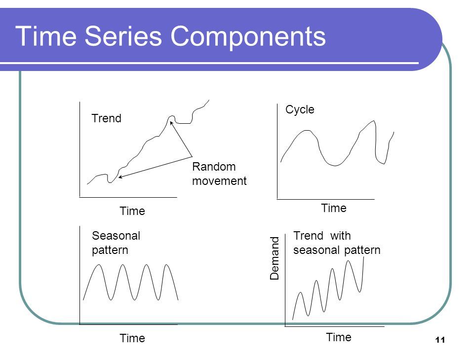
In time-series data, trend, seasonal and cyclic are three important components to be looked at.
Trend:
When there is a long-term increase or decrease, you call it a trend. A trend is said to be changing direction if it becomes decreasing trend from an increasing trend or vice versa. A trend need not be linear. Beware, sometimes it is just a part of a seasonal/cyclic pattern.
Eg.: Traffic of AnalyticsVidhya website.
Seasonal:
When a time series data is affected by a seasonal factor, say a month, time of the year, or the day of the week, it is called a seasonal pattern. In simple terms, you can call it seasonal when the data is influenced by some sort of calendar factor, say monthly or quarterly. The frequency is always known and fixed.
Eg.: Sales at a Clothing store is usually at their peak during the festive season and are back to normal once it is over. And it repeats every year.
Cyclic:
When the rises and falls exhibited by data are not of fixed frequency, it is said to be seasonal. These fluctuations are mainly due to economic conditions, and they are often related to the ‘business cycle’. A business cycle is usually of 3 years.
They are usually lengthier than a seasonal component and their magnitude is much higher than the seasonal component.
Noise:
The randomness in data.

A series is an aggregate or combination of two or more of the time series components. When all series have level and noise, trend and seasonality are optional. The components could either be combined additively or multiplicatively.
Additive Model:
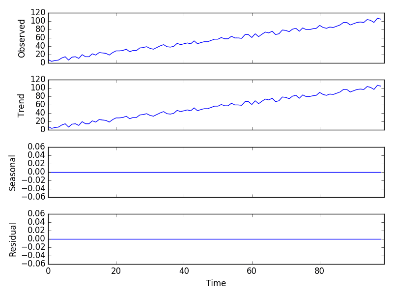
In this type of model, the components are combined by addition and the trend is linear. The changes over time are consistently made by the same amount. The seasonality is supposed to have the same frequency (width of cycles) and amplitude (height of cycles) over time.
y(t) = Level + Trend + Seasonality + Noise
We take numbers from 1 to 99 and randomly add a number between 0 and 9 with that to include randomness in our time series data.
from random import randrange
from pandas import Series
from matplotlib import pyplot
from statsmodels.tsa.seasonal import seasonal_decompose
series = [i+randrange(10) for i in range(1,100)]
result = seasonal_decompose(series, model='additive', period=1)
result.plot()
pyplot.show()

Multiplicative Model:
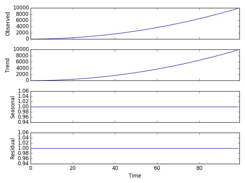
In this type of model, the components are combined by multiplication and is nonlinear. Changes tend to increase or decrease over time. The seasonality increases or decreases in frequency and/or amplitude over time.
y(t) = Level * Trend * Seasonality * Noise
We square the numbers from 1 to 99 and use as a time series data.
|
|
from pandas import Series from matplotlib import pyplot from statsmodels.tsa.seasonal import seasonal_decompose series = [i**2.0 for i in range(1,100)] result = seasonal_decompose(series, model='multiplicative', period=1) result.plot() pyplot.show() |
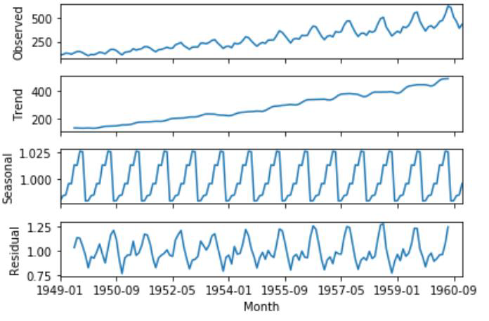
Let us take the AirPassengers data and try to decompose it into time series components.
from matplotlib import pyplot
from statsmodel.tsa.seasonal import seasonal_decompose
series = pd.read_csv("AirPassengers.csv", header = 0, index_col = 0)
result = seasonal_decompose(series, model = "multiplicative" , frequency = 10)
result.plot()
pyplot.show()
Conclusion
In this article, we have seen some basic terms of time-series forecasting and examples of the same. I’m Keerthana, a data science student fascinated by Math and its applications in other domains. I’m also interested in writing Math and Data Science related articles. You can connect with me on LinkedIn and Instagram. Check out my other articles here and here.


