Convolution Neural Network – Better Understanding

This article was published as a part of the Data Science Blogathon

Introduction:

In the world of Deep Learning (DL), there are many trending and advanced models are emerging, for making our life (researchers!) easy. One among them is Convolution Neural Network (CNN), in this article we are going to see in detail this model.

Deep Learning -The Evolution:

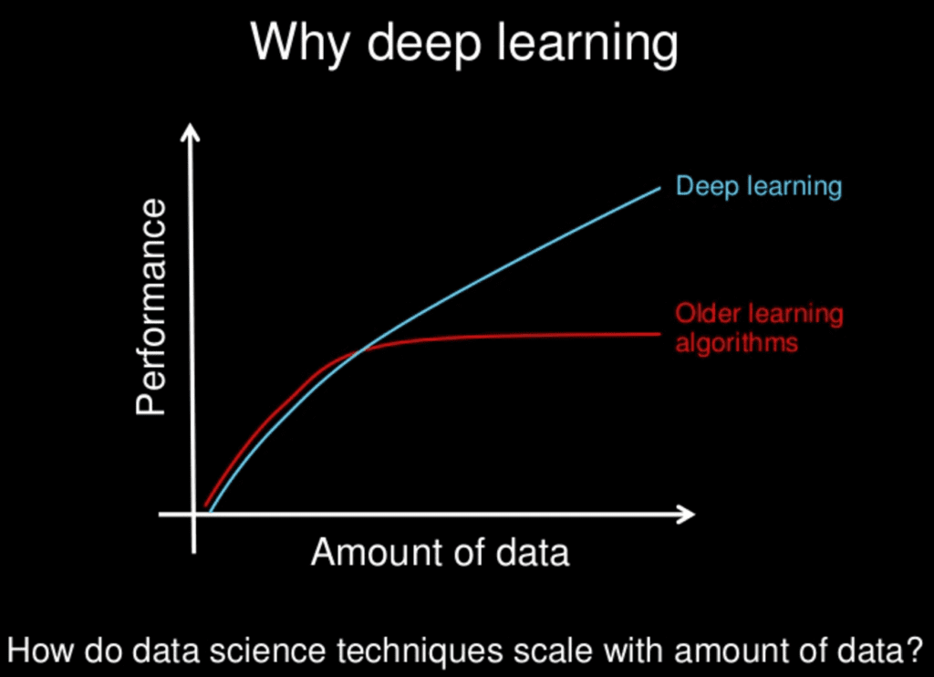
In today’s scenario, many people irrespective of their domain (degree qualification!) opt for the Data Science domain. There may be much reason but the ground reality is most of the IT giants and big organization, they are shifting towards DATA SCIENCE side with a small part (means along with the current speciality, they also include data science ) or as a full time. One of the main reasons is smartness and also its robustness irrespective of any domain. If you look into the history behind Deep Learning it is not the technology that happened before some five or ten years old. In 1943, Walter Pitts and Warren McCulloch created a computer model based on the human brain’s neural networks. They used algorithms and mathematics, called “threshold logic” to mimic the thought process. But the popularity gets faded in the middle years, you know because of two simple reasons,

1. Availability of data (more and more data!)

2. Processor power (to run the loads and loads of data!)

Geoffrey Hinton – Father of Deep Learning

In simple terms, Deep Learning is used to mimic our very own Human Brain (On Processing! but not fully!) and to replicate, how well our human brain learns things faster and thinks with sense.

Still need to read more about the DL approach, (https://www.tango-learning.com/post/deep-learning-an-intuition-behind-the-technology)

Types of Deep Learning:

There are many different types of DL as per different sources prevailing in our internet ocean, but predominately, DL is classified as,

1. Artificial Neural Network (ANN)

2. Convolution Neural Network (CNN)

3. Recurrent Neural Network (RNN)

Artificial Neural Network:

We discussed already Artificial Neural Network (ANN) in detail in the following article with python code. Please find the link for better understanding,  (https://www.analyticsvidhya.com/blog/2021/06/artificial-neural-networks-better-understanding/)

Convolution Neural Network – Understanding:

Before getting into the main topic, Convolution Neural Network (CNN). First, let us understand some basic clarity, so look into the below picture,

Image Source: Google Image

What we inferred from the above diagram? Some say it as Men and some say it as Women and some say it as both!.. Because of the features that get picked by our brain while viewing the drawing. If you would easily differentiate the above picture, then view the next one, the below-mentioned picture,

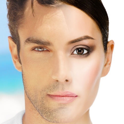
It’s actually a fusion of the male and female picture while viewing some thought as male and female. So above two examples illustrate to us how the brain works, that it processes certain features on these examples or whatever we see in real-life and it classifies that as such. So we are going to do the same process with Neural Network with CNN is almost very similar. It’s like how we are getting features from the above pictures, in the same way, the computers also going to process, sounds interesting right!

Yann Lecun – Grandfather of Convolution Neural Network!

Convolution Neural Network – Layman Understanding:

As human psychology, when we sit or lie on a bed or in any position (when we are awake – condition applied!), we tend to observe and look at our surroundings with or without knowledge, our brain will be in an active state only and it keeps on processing and sometimes it keeps predicting too right!.

Just look at the above picture, what we identified from the photo is some persons and some projects are present. After that what we analyzed are plates with some food not in particular and tumbler with water, then ID card, etc…Added in the emotional side if we observe means it’s a happy moment with friends and randomly enjoying some poses. Whatever mentioned above, are predictions by seeing the pictures,  so how is possible to predict? Then how you can find the objects and emotion predictions? Our eyes and our brain work in perfect harmony to create such beautiful visual experiences. The system which makes this possible for us is the eye, our visual pathway, and the visual cortex inside our brain.

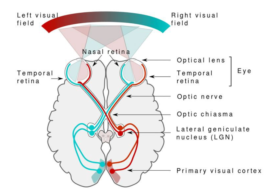
Lights and colours on the retina are captured in our eyes. These signals cross the receptors of the retina to the optical nerve and are transferred to the brain for this information to be meaningful. The eye and the visual brain are extremely complex and hierarchical. In perceiving and understanding what we around us view, the full visual path plays a vital part. It is this mechanism inside of us that allows us to understand the image above, the text of this essay, and every other work we do daily. So these processes we are doing from our childhood and so we can predict and analyze through eyes and brain coordination.

So the same process, is that possible for computers? and the simple answer is YES!. computers can SEE the world but in a different way – through numbers. Like the picture below,

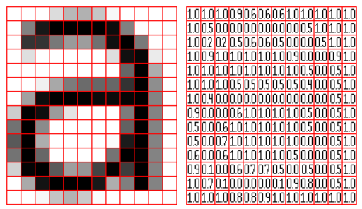
The importance of layers of neurons arranged in each algorithm is, each layer concentrates each pattern and its importance like firstly it observes simple patterns such as lines, curves, then some complex patterns like texts, objects, and face and more complex patterns present in the image or whatever inputs that we are analyzing. This process is almost like a human’s point of view when we are randomly visualizing or seeing anything our brain analyzes any input like this only but in a matter of very few seconds.

So there are various steps to achieve this CNN algorithm, they are as follows,

1. Convolution layer

2. Activation function (ReLu layer)

3. Pooling

4. Flattening

5. Full connection

On the whole, the below animation will explain how CNN works,

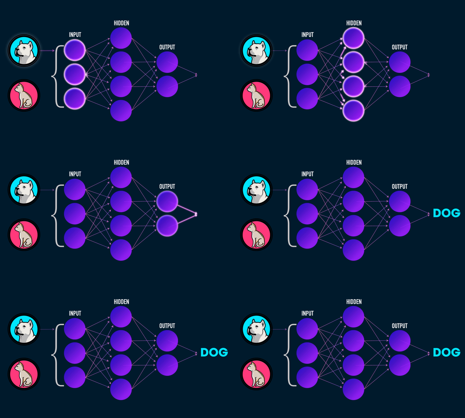
another interesting visualization,

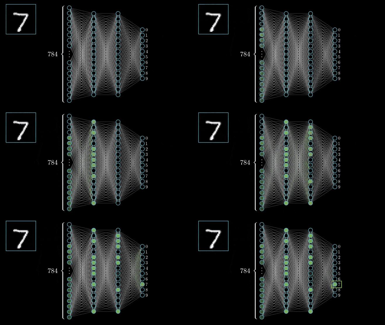
Let’s see one by one what the steps explain or conveys,

1. Convolution Layer:

The most important portion or segment in the CNN algorithm. The mathematical notation of Convolution is as follows,

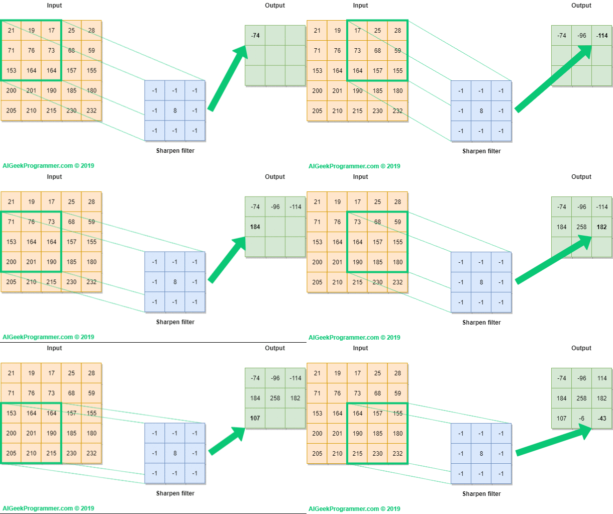
here in the above equation, we can infer that convolution is an integration of two simple functions (f and g). We have two terms, one is our input/dataset in matrix format and another one is feature detector or kernel or filters (it will be 3*3 or 5*5 or 7*7 matrix, depends on the architecture that we are using!) when compared to the input image matrix, this matrix is smaller but we can get deeper knowledge from this kernel part only.

Consider an input and kernel matrix as

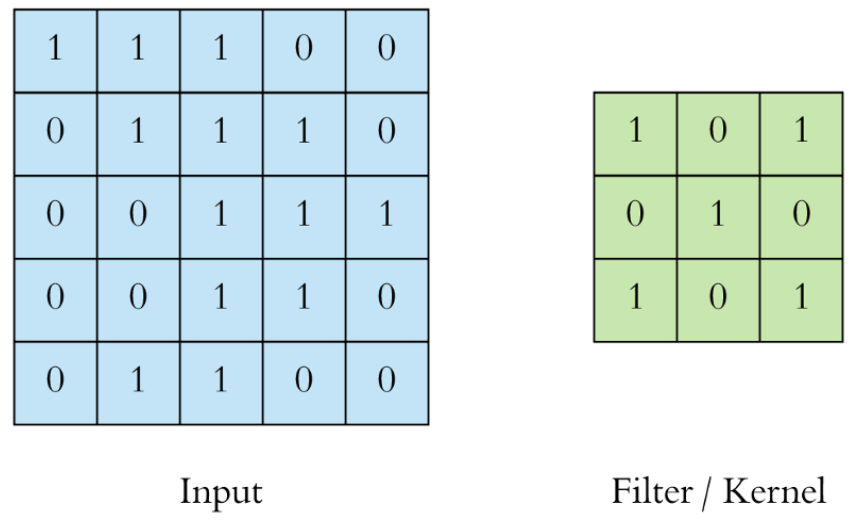
The first step in convolution function is kernel matrix shown above figure, which slides through input image as,

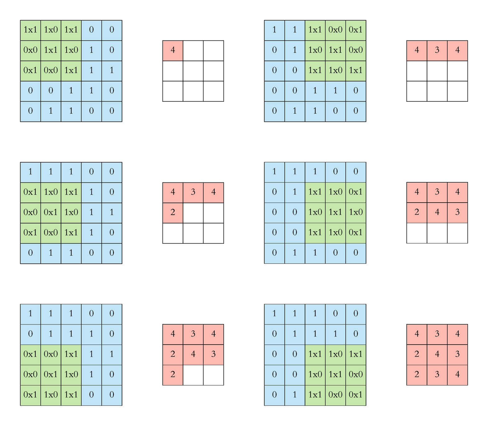
In a static way, we can explain the above step as,

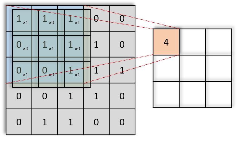
If you note clearly, the value 4 in the output matrix, which depends on the 9 values of 3*3 matrix and another importance is the value doesn’t change if any position of the value of the input matrix changes too. This is the RECEPTIVE FIELD of this output value, meaning the importance of the neuron layer to find a particular object or text or anything. Each value in the output value or matrix is sensitive to only a particular region, and hence we need to use our kernel matrix wisely depends on applications.

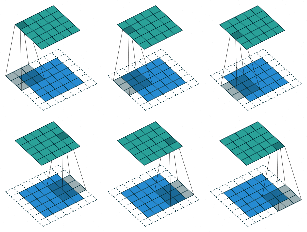
In a more layman way, convolution process `like,

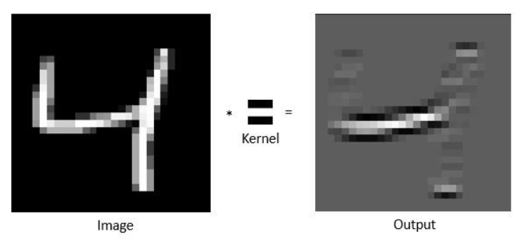
For a change, let’s consider handwritten digits for a little more understanding through some pictures (as I believe the picture speaks 1000 words!). So here, in the below figure, I need to concentrate only horizontal lines alone, so for this with the help of kernel matrix I can get the output matrix as,

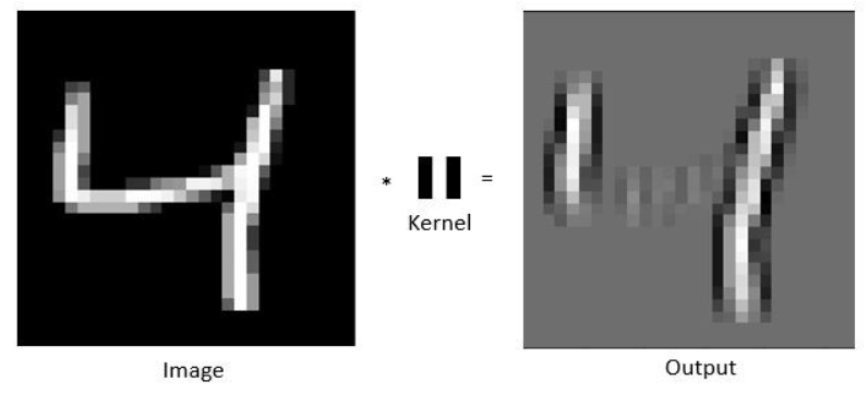
In the same way, if I need to concentrate with respect to the vertical lines, in the same way by using kernel matrix, I can able to get the output values as,

So from all the explanations above, what we infer from this CONVOLUTION block, extraction of important terms, or technically we call it feature extraction. So convolution block is used to achieve feature extraction from the given dataset by avoiding other unimportant features or dimming or avoiding useless information or feature in simple.

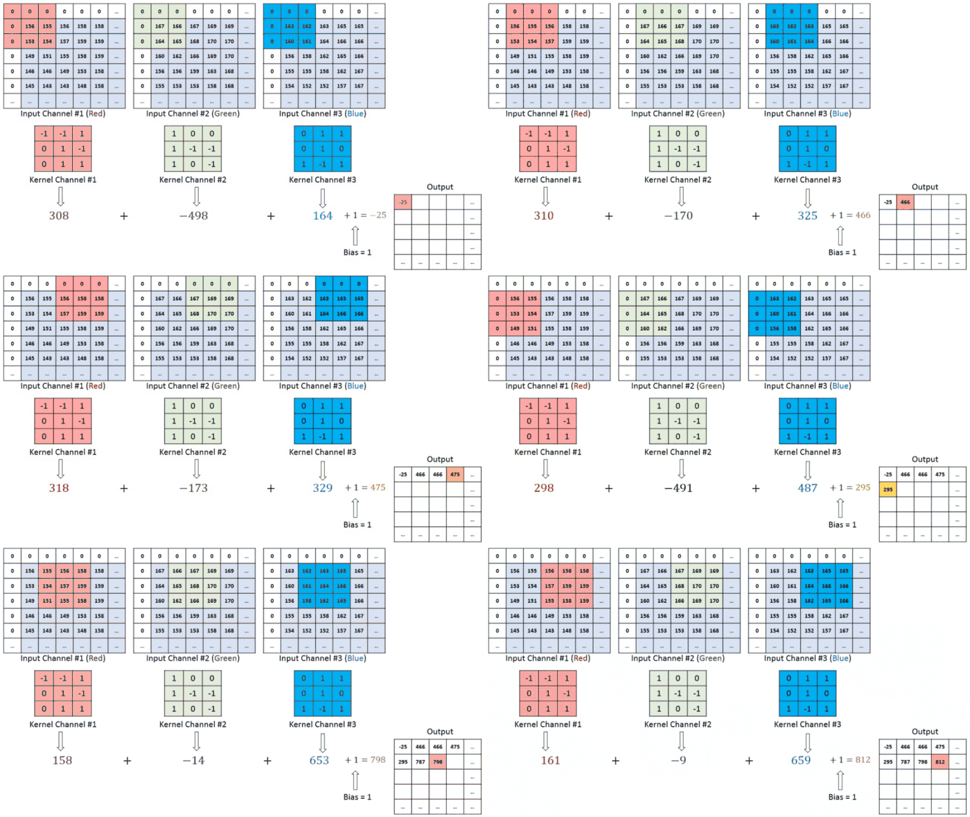
Filters play’s an important role in transforming the data (numbers/pixels), the resultant output we call activation maps, which means regions where features specific kernel to be detected from the input data. Dimension of feature map = Dimension of filter

In the case of an image, convolution layer works like, because of RGB format wrt image,

2. Activation Function:

So once the convolution process gets over for our input dataset (sliding process!), the next important step to proceed in the CNN algorithm is the activation function.

When comparing with a neuron-based model that is in our brains, the activation function is at the end deciding what is to be fired to the next neuron. It takes in the output signal from the previous cell and converts it into some form that can be taken as input to the next cell. It’s a non-linear transformation that we do for inputs that we receive before sending them to the next layer or neuron. AF is also known as Transfer Function. For further information about AF visit the following link (https://www.analyticsvidhya.com/blog/2021/06/artificial-neural-networks-better-understanding/)

Let’s consider the same example as we have seen for the handwritten digit dataset, after the convolution process, we have passed AF (ReLU), then the output will be like,

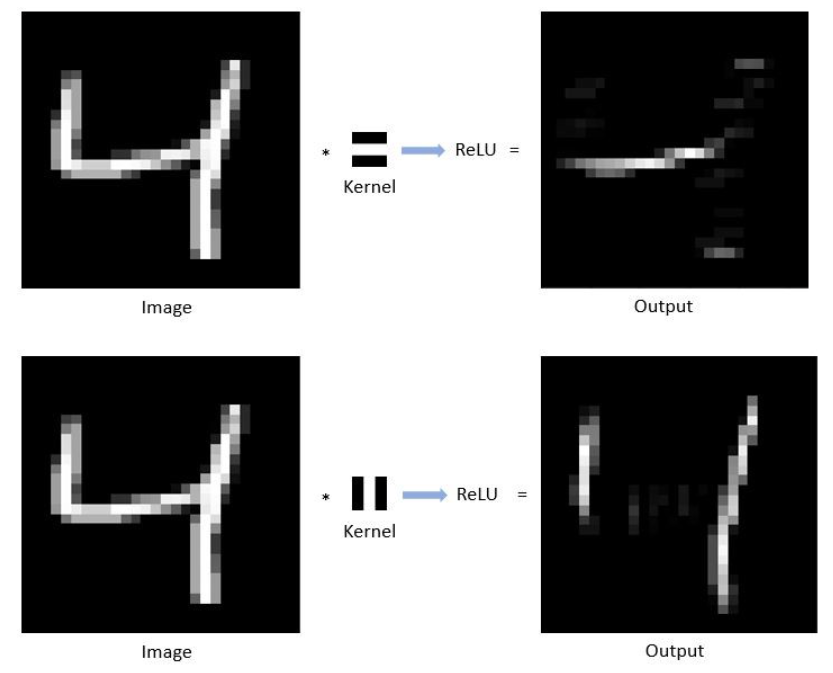
So what you infer from this AF process, the output that we got from the convolution process in general one means it has some or few unwanted information, depending upon the kernel filter or matrix that we used. Here in AF, useful information is passed on to the next process. It’s just transferring the information to the next process.

3. Pooling:

We all know the importance of swimming pool right – stress buster, if we do swimming for an hour, whatever stress we have it will be gone, in the same way, Pooling process which means it reduces the dimensionality of our matrix. The main importance of pooling is to reduce overfitting and computation in our dataset. In a layman level, pooling can be explained by,

The main importance of the pooling layer is to detect the edges, corners and in application-like images, it can be used to detect facial features like nose, eyes by using multiple filters. It’s like filtering the feature map, because we get the feature map from the convolution process, and here in pooling we are going to apply it to the filter. Mostly the size of the filter is 2*2, which means in the pooling process feature map gets reduced by the factor of 2 (in simple reduced by half of the feature map dimension), intern it reduces each value in the feature map to one quarter.

It has two main types, Max-Pooling and Avg-Pooling.

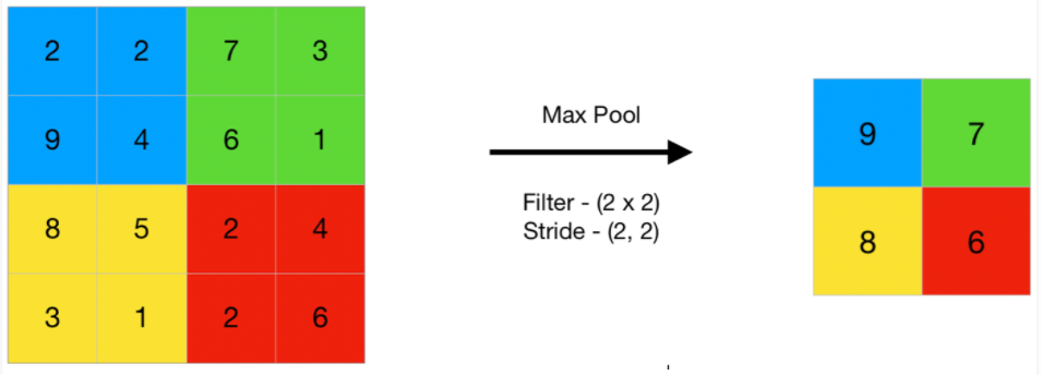
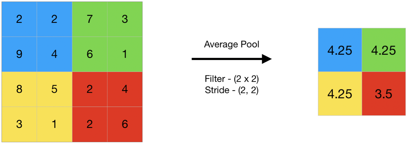
and some other types of pooling are as follows, firstly will see a minimum pooling,

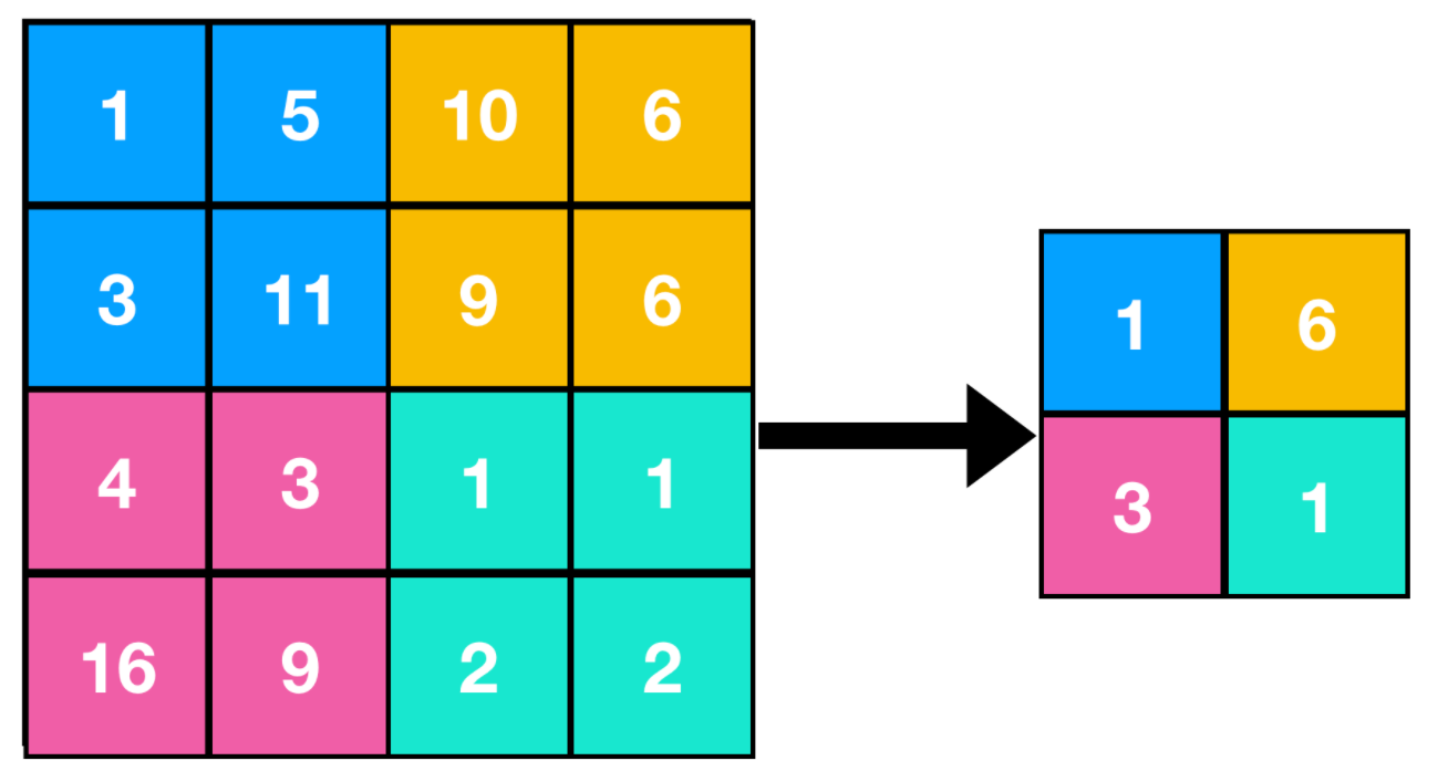
and lastly adaptive pooling, herein the user doesn’t need to manually define hyperparameters, it needs to define only output size, and the parameters are picked up accordingly

In a more understanding, let’s consider a cat image in a different position as like this figure,

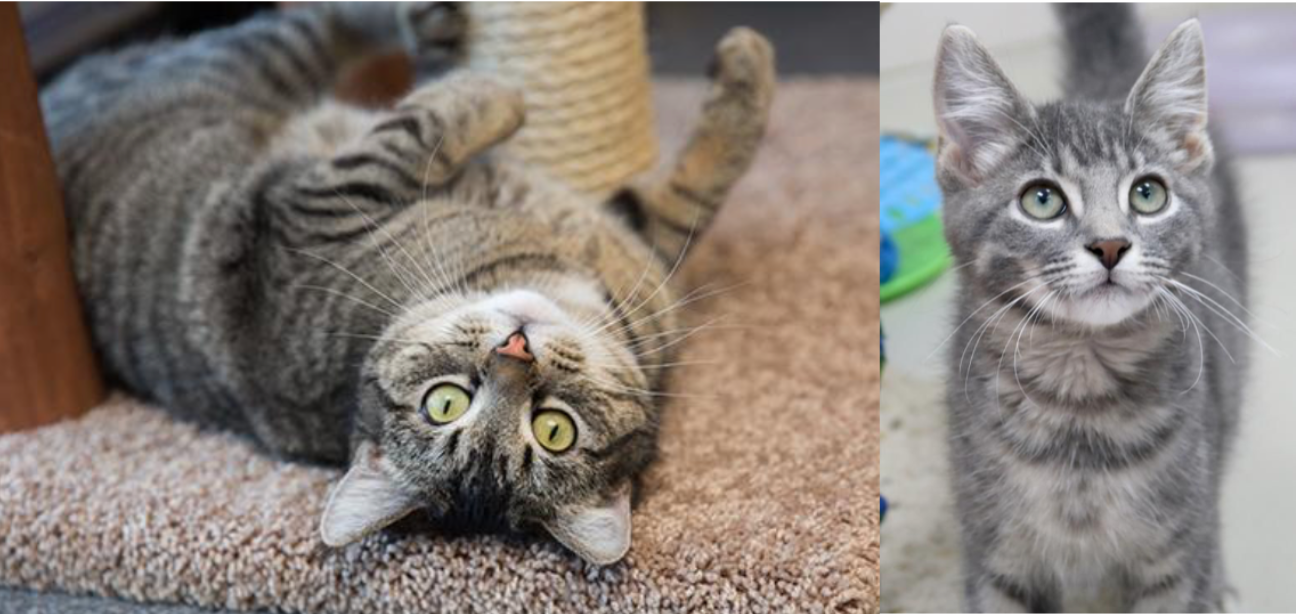
The importance of the convolution layer is to find the feature extraction or location of features through feature maps. But in the above figure if I apply the convolution it may get confused because the first half of the image is in reverse position, so here comes the pooling process, apart from the reduction process it also helps in Translational Invariance (ability to ignore the position shifts).

There are some important terms to be noticed in the Pooling process,

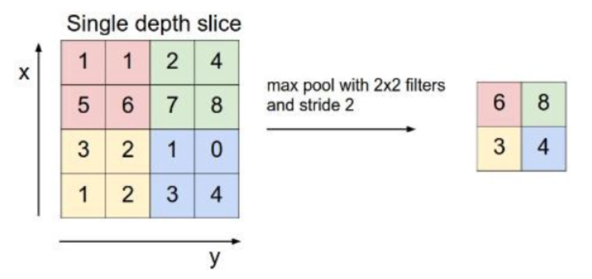
1. Filter Size – Describes filters size like 2*2 or 3*3 or anything

2. Stride – describes the number of steps filter takes while traversing the image

3. Padding – Sometimes filter size creates a border effect in the feature map, the effect can be overcome through padding.

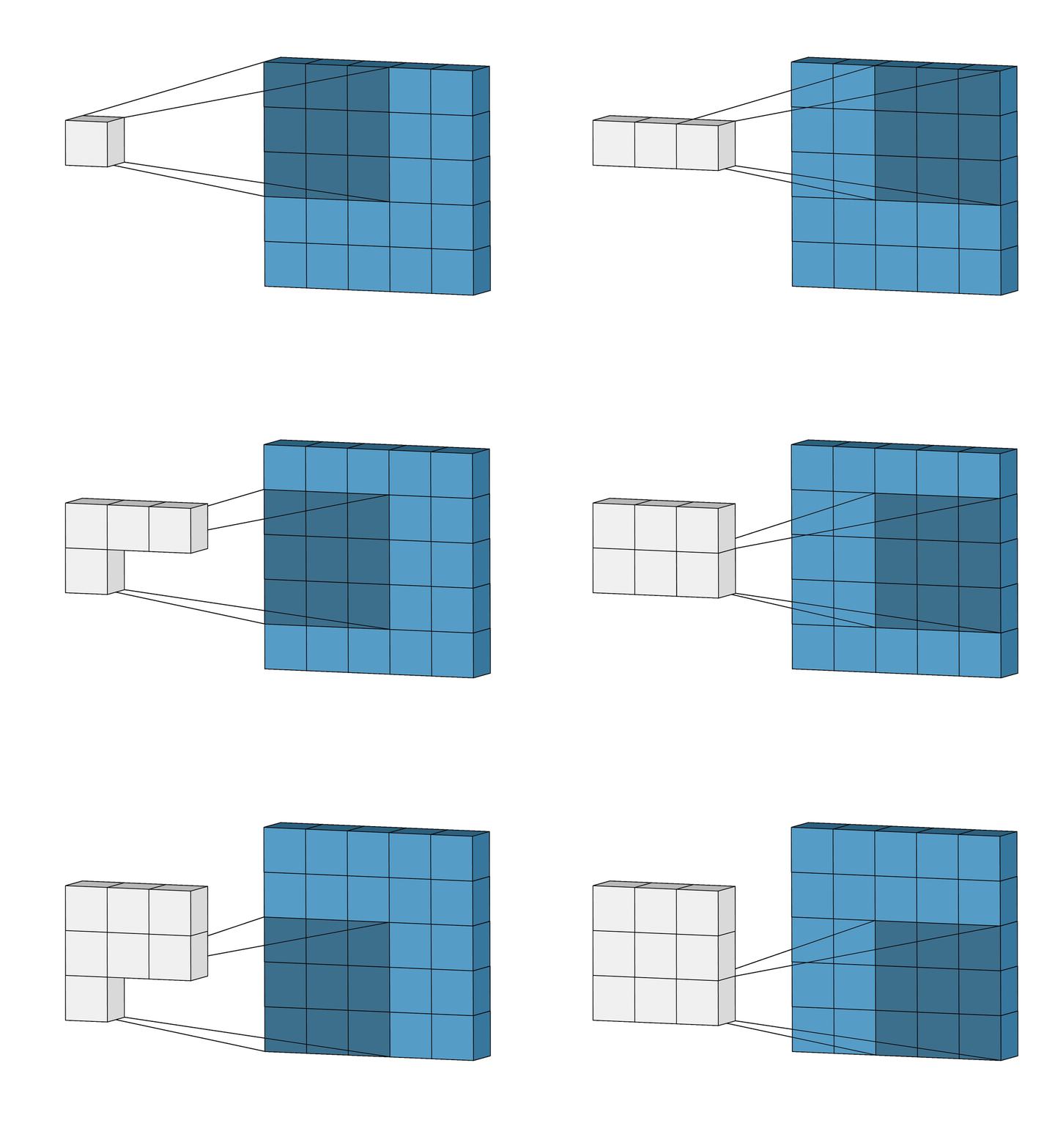
If you notice in the above figure, the filter size is 3*3, stride size is 1.

4. Flattening: 

So the next layer after the pooling process is flattening, here in this process, we are going to make our matrix into a single column, basically, we are taking row by row numbers and put them into a single column.

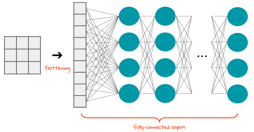
And the importance of making them into a single column is simple, the next step is to feed them to the neural network for further processing.

Flattening is converting the data into a 1-dimensional array for inputting it to
the next layer. We flatten the output of the convolutional layers to create a
single long feature vector. And it is connected to the final classification
model, which is called a fully connected layer.
In other words, we put all the pixel data in one line and make connections with
the final layer. And once again. What is the final layer for? The
classification of ‘the cats and dogs’ or normal and abnormal, good or bad, or
any classification.

5. Full Connection / Fully Connected layer: 

Last layer, in which each pixel or each number/point is considered as a separate neuron just like a NN. The last fully-connected layer will contain as many neurons as the number of classes to be predicted.

Now that we have converted our input image into a suitable form for our Multi-Level fully connected architecture, we shall flatten the image into one column vector. The flattened output is fed to a feed-forward neural network and backpropagation is applied to every iteration of training. Over a series of epochs, the model can distinguish between dominating and certain low-level features in images and classify them.

This layer assigns random weights to the inputs and predicts a suitable label

Apart from these blocks, there are also some special blocks used for CNN,

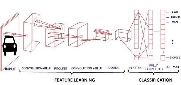
Fully Connected Output layer:

The final layer of the CNN model contains the results of the labels determined for the classification and assigns a class to the dataset (input)

Softmax

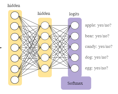
The reason why softmax is useful is that it converts the output of the last layer in your neural network into what is essentially a probability distribution. It is mainly used to normalize neural networks output to fit between zero and one. It is used to represent the certainty “probability” in the network output.

Dropout

The main idea behind using dropout is simple, to avoid overfitting. The most popular regularization method is used in Neural networks. Even if we are using a different model and achieve around 90% of accuracy, by using dropout we can able to achieve around 92% of accuracy.

During training time, at each iteration, a neuron is temporarily “dropped” or disabled with probability p. This means all the inputs and outputs to this neuron will be disabled at the current iteration. The dropped-out neurons are resampled with probability p at every training step, so a dropped-out neuron at one step can be active at the next one. The hyperparameter p is called the dropout rate and it’s typically a number around 0.5, corresponding to 50% of the neurons being dropped out.

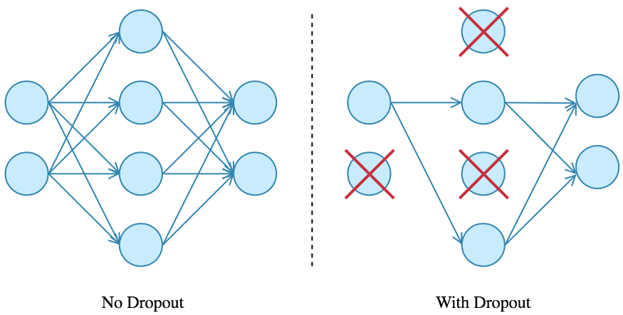
Almost all state-of-the-art deep networks now incorporate dropout. There is another very popular regularization technique called batch normalization

Summary of CNN:

1. Provide the data/dataset (any format of data) into the convolution layer

2. Take convolution with featured kernel/filters

3. Next apply a layer, Pooling for reducing the dimensions

4 If you need a deeper understanding add these layers repeatedly.

5. Next step is to apply to flatten for a single column

6. Feed into a fully connected layer

7. Now lastly train the model with appropriate metrics and optimizer

CNN – Different Architecture Models

Before getting deeper into the models, let’s understand some basic terminologies,

1. Wider – means more feature maps (filters) in the convolutional layers

2. Deeper – means more convolutional layers

3. High Resolution – means that it processes input images with larger width and depth
(spatial resolutions). That way the produced feature maps will have a higher
spatial dimensions.

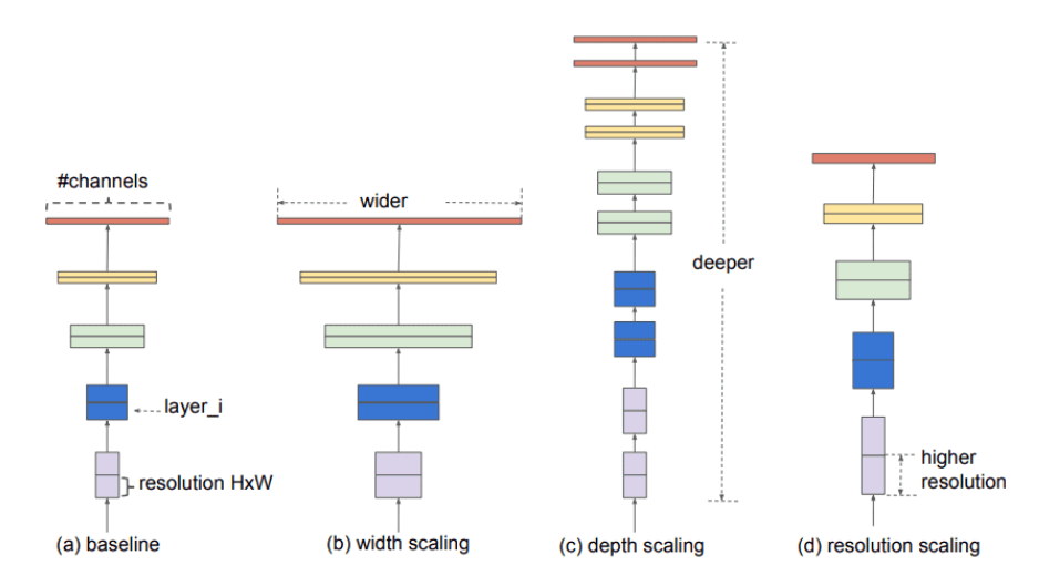
Based on the architecture of layers that we have seen so far with some technical terms, CNN is categorized into different models, some of them are as follows,

1. LeNet-5 (2 – Convolution layer & 3 – Fully Connected layers) – 5 layers

2. AlexNet (5 – Convolution layer & 3 – Fully Connected layers) – 8 layers

3.  VGG 16 (13 – Convolution layer & 3 – Fully Connected layers) – 16 layers

4. Inception V1 – 22 layers

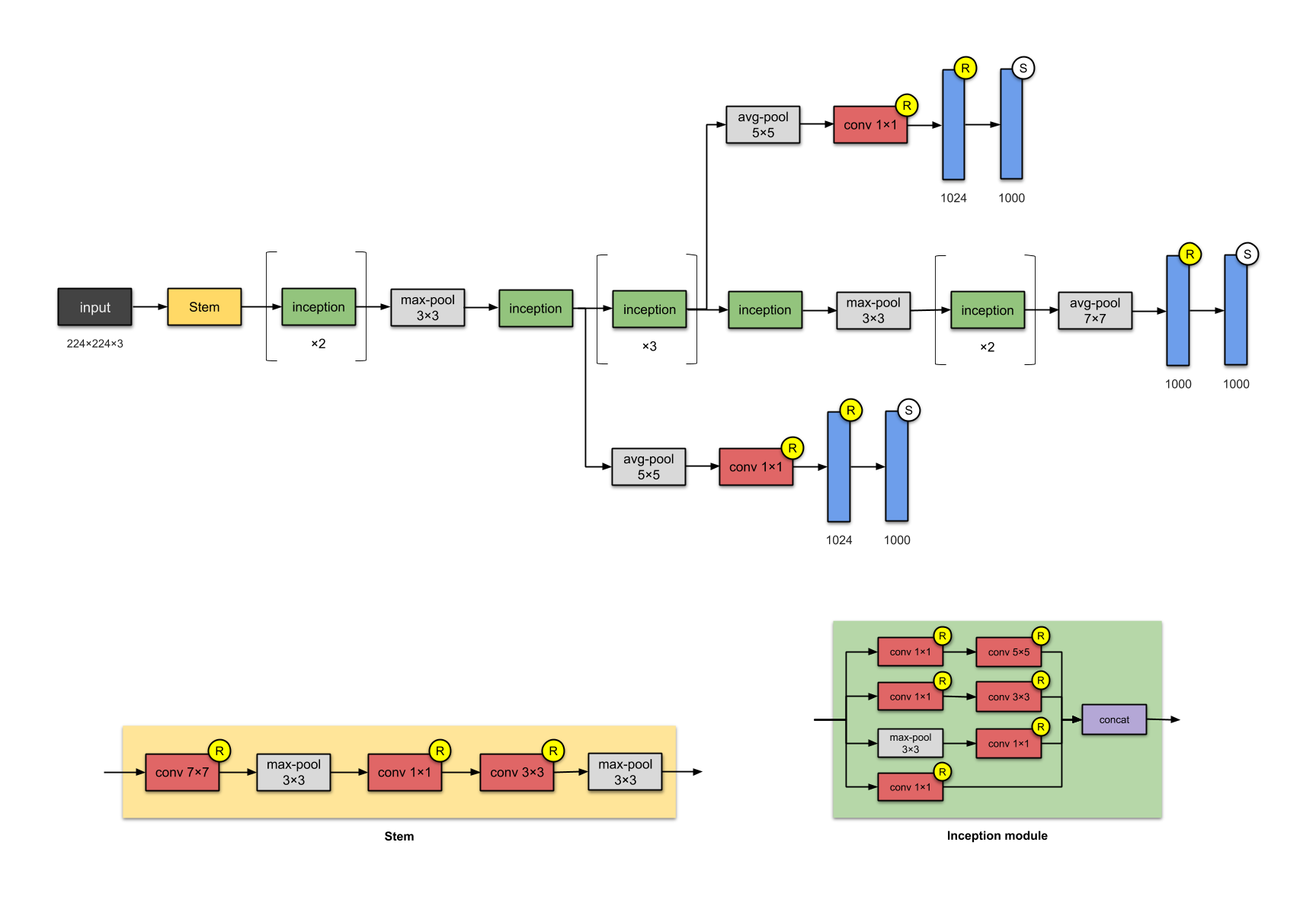
5. Inception V3

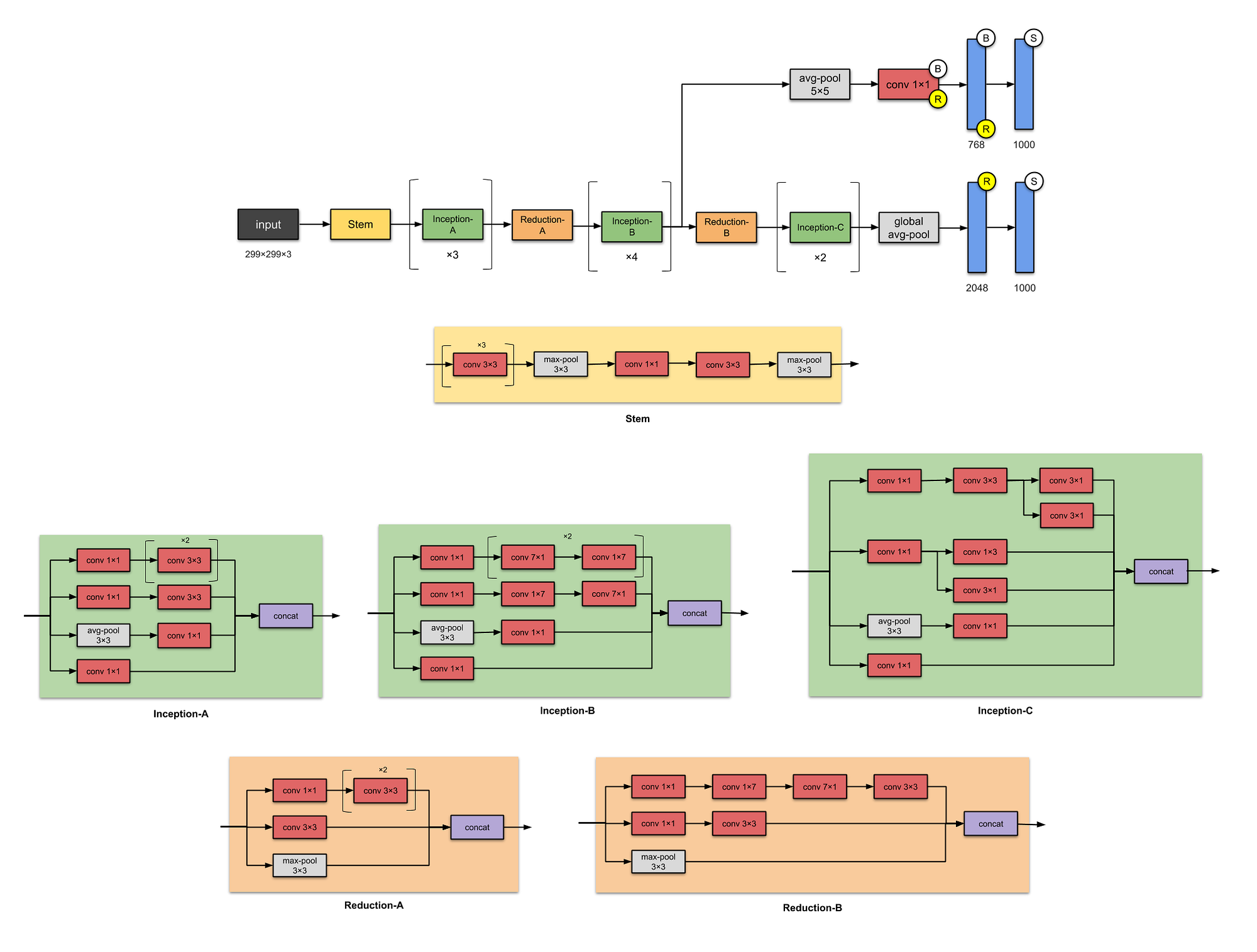
6. ResNet 50

7. Xception

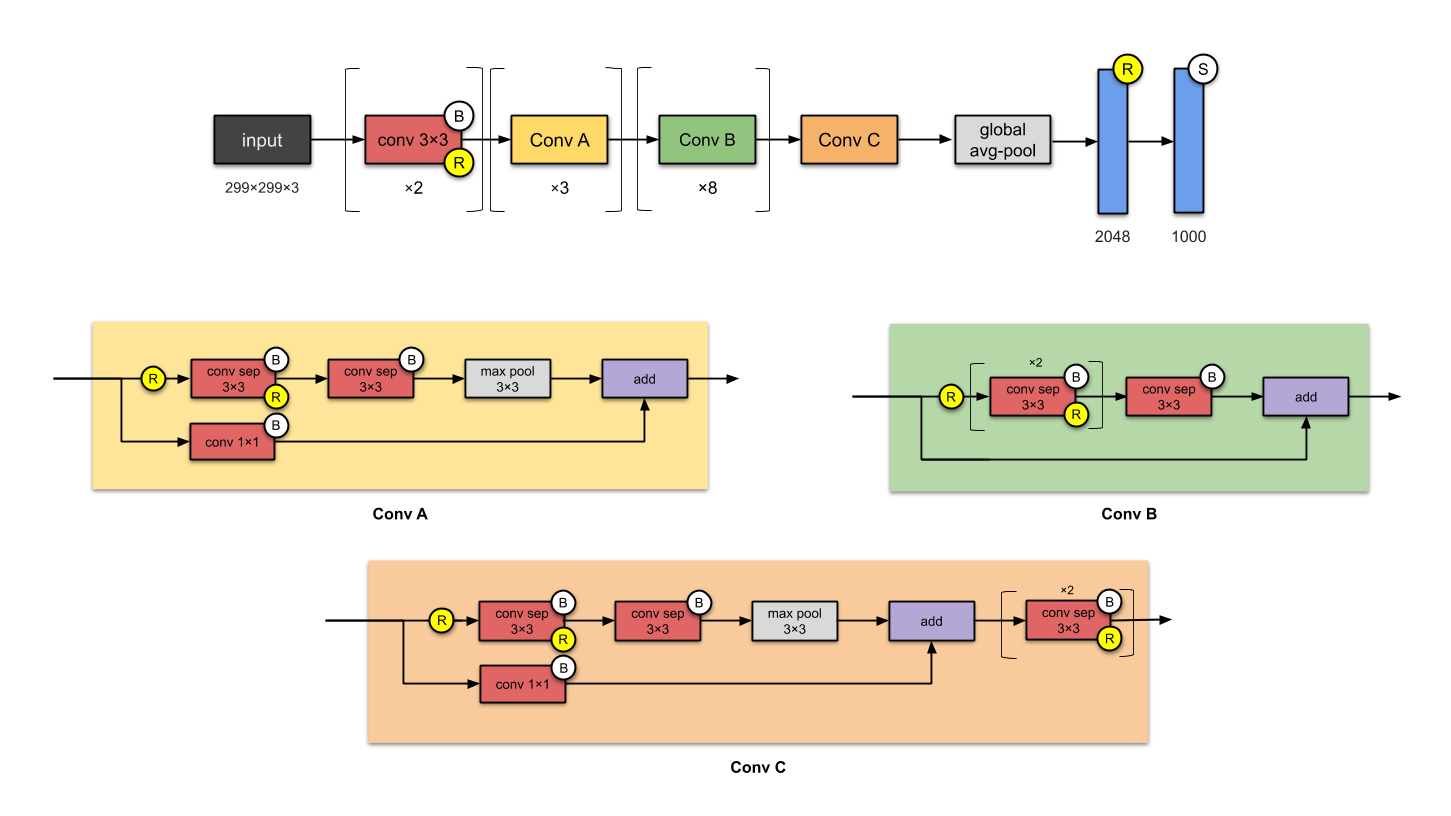
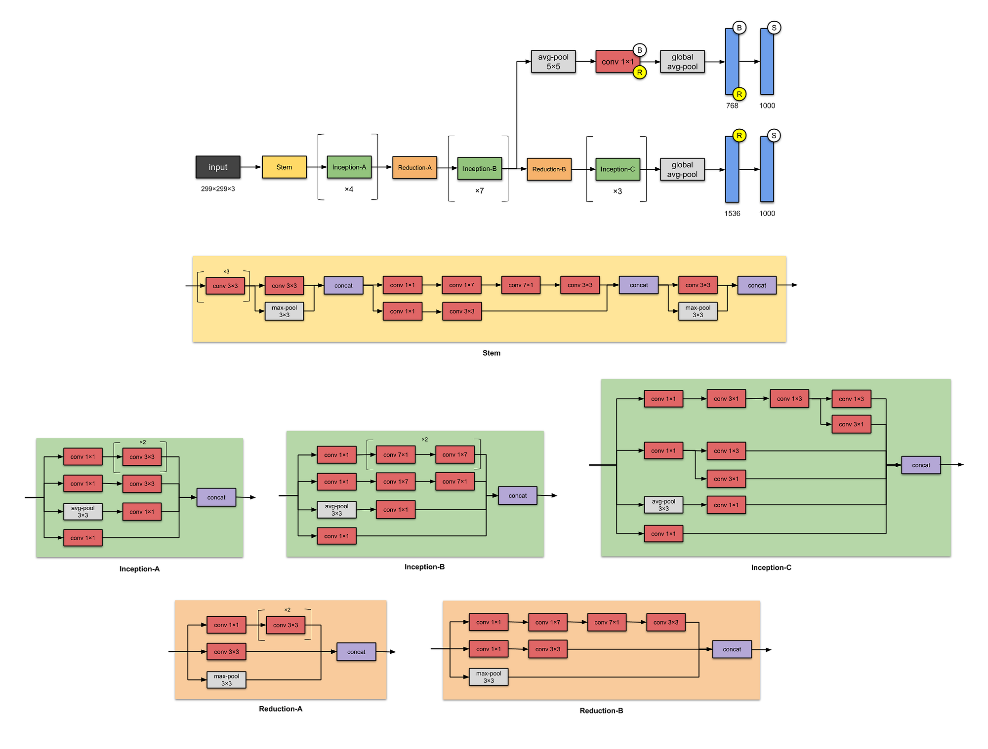
8. Inception V4

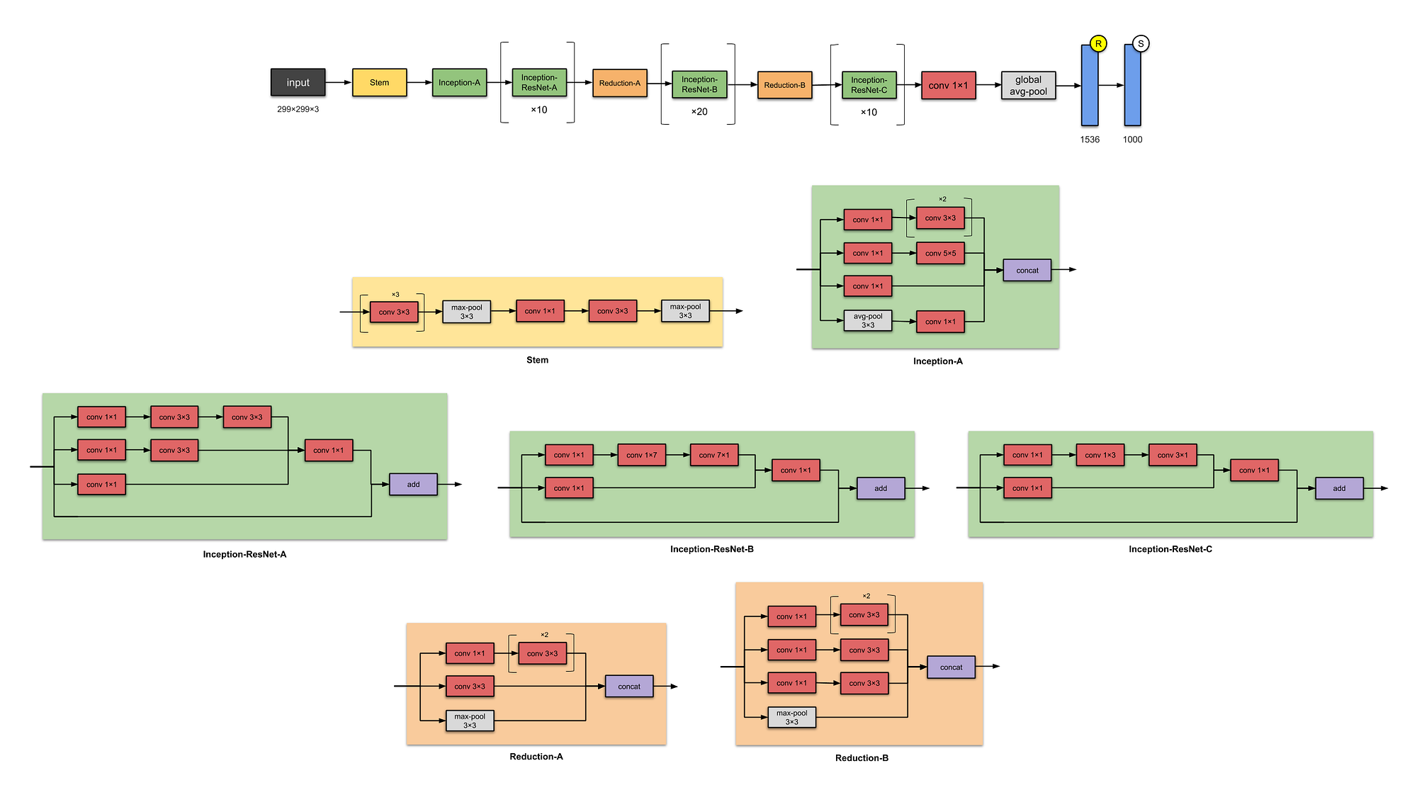
9. Inception ResNet V2

10. ResNeXt 50

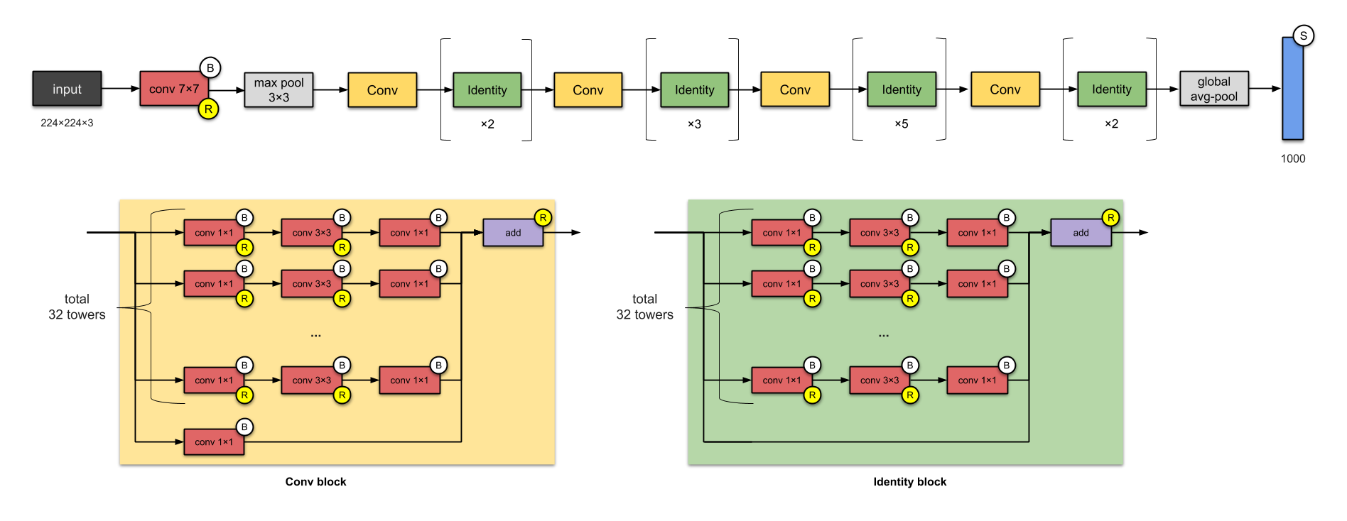
All the pictures are taken from https://towardsdatascience.com/illustrated-10-cnn-architectures-95d78ace614d 

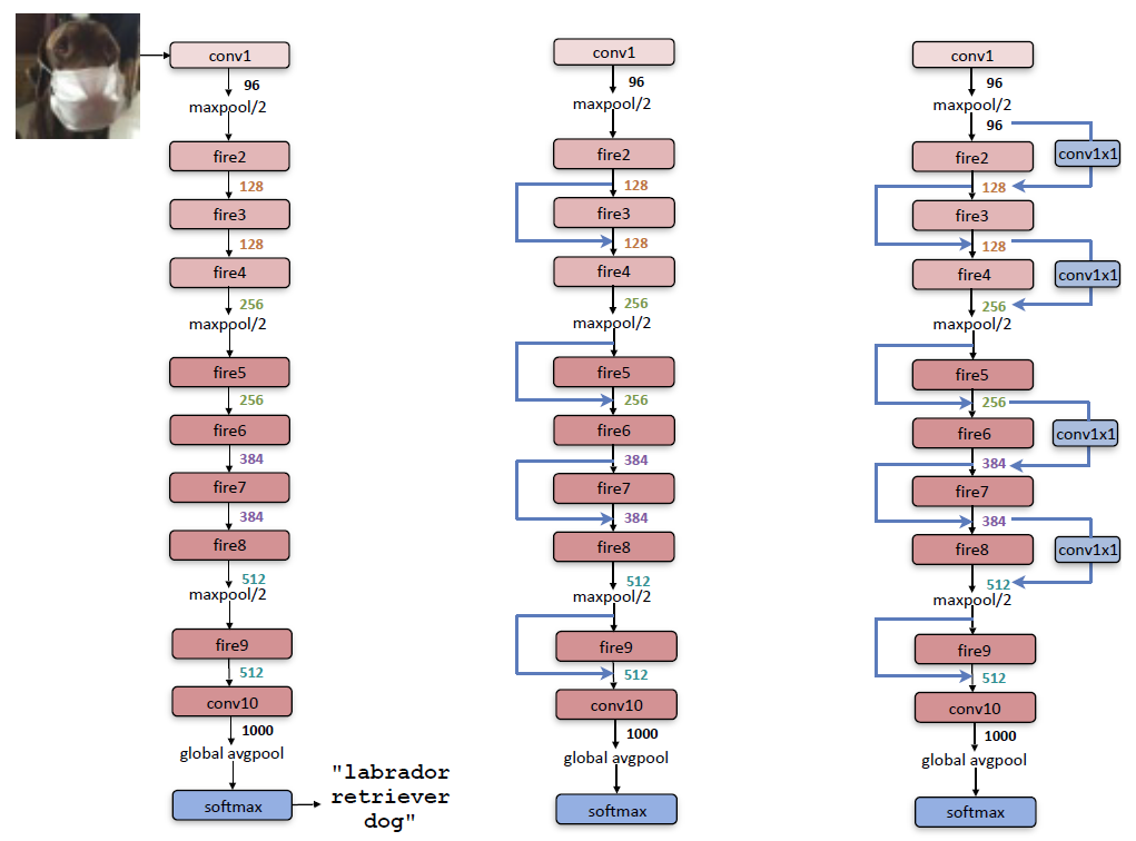
11. Squeeze Net

12. Dense Net

Image Source: https://towardsdatascience.com/paper-review-densenet-densely-connected-convolutional-networks-acf9065dfefb

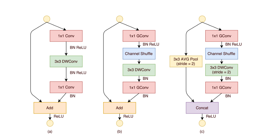
13 Shuffle Net

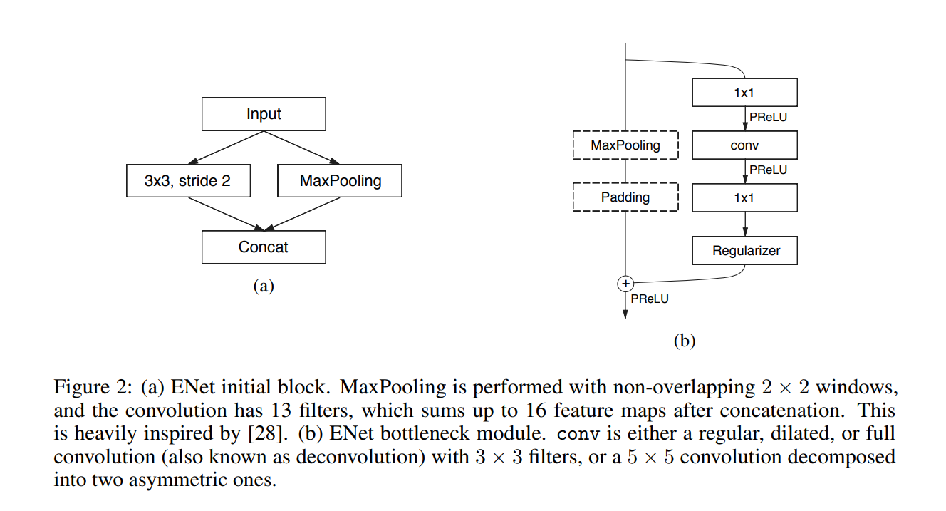
14 ENet

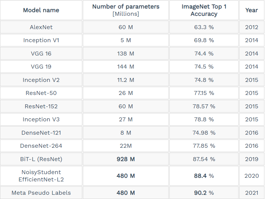
Some of the most famous model comparisons are shown below,

Advantage of CNN:

1. Automatically detects important features without any human supervision

2. Computationally efficient (Convolution and Pooling process performs parameter sharing)

3. Weight Sharing

4. High Statistical efficiency

5. Translational Invariance

Disadvantages of CNN: 

1. Classification of Images with different Positions (different angles, different backgrounds, different lighting conditions)

2. Adversarial examples (CNN takes an image along with some noise it recognizes the image as a completely different image whereas the human visual system will identify it as the same image with the noise)

3. Coordinate Frame (Coordinate frame is basically a mental model which keeps track of the orientation and different features of an object)

4. Slower due to functions like Maxpool

5. As several layers are functional then the training process takes lots of time if our CPU doesn’t have a good GPU

These drawbacks lead to the formation of the Capsule Neural Network

Application of CNN:

1. Decoding Facial Recognition

2. Analysing Documents

3. Classification

4. Segmentation (Organs or any anatomical structures is a fundamental Image Processing technique for Medical Image Analysis)

5. Detection (Common task for Radiologist is to detect abnormalities with Medical Images)

Python Coding with CNN

I hope you understand some bit about CNN from the above explanation and some visualization,

 Dataset: CIFAR 10 Image Classification

#importing basic libraries

import tensorflow as tf

import matplotlib.pyplot as plt

#importing default dataset

from tensorflow.keras.datasets import cifar10
#loading dataset

# setting class names from dataset

class_names=['airplane','automobile','bird','cat','deer','dog','frog','horse','ship','truck']

#loading the dataset

(x_train,y_train),(x_test,y_test)=cifar10.load_data()

#normalizing train data

x_train=x_train/255.0

x_train.shape

#normalizing test data

x_test=x_test/255.0

x_test.shape
#random check dataset

plt.imshow(x_test[222])

#Building CNN model

cnn_model=tf.keras.models.Sequential()

# First Layer

cnn_model.add(tf.keras.layers.Conv2D(filters=32,kernel_size=3,padding="same", activation="relu", input_shape=[32,32,3]))

# Second Layer

cnn_model.add(tf.keras.layers.Conv2D(filters=32,kernel_size=3,padding="same", activation="relu"))

# Max Pooling Layer

cnn_model.add(tf.keras.layers.MaxPool2D(pool_size=2,strides=2,padding='valid'))

# Third Layer

cnn_model.add(tf.keras.layers.Conv2D(filters=64,kernel_size=3,padding="same", activation="relu"))

# Fourth Layer

cnn_model.add(tf.keras.layers.Conv2D(filters=64,kernel_size=3,padding="same", activation="relu"))

# Max Pooling Layer

cnn_model.add(tf.keras.layers.MaxPool2D(pool_size=2,strides=2,padding='valid'))

# fifth Layer

cnn_model.add(tf.keras.layers.Conv2D(filters=128,kernel_size=3,padding="same", activation="relu"))

# Sixth Layer

cnn_model.add(tf.keras.layers.Conv2D(filters=128,kernel_size=3,padding="same", activation="relu"))

# Max Pooling Layer

cnn_model.add(tf.keras.layers.MaxPool2D(pool_size=2,strides=2,padding='valid'))

# Flattening Layer

cnn_model.add(tf.keras.layers.Flatten())

# Droput Layer

cnn_model.add(tf.keras.layers.Dropout(0.5,noise_shape=None,seed=None))

# Adding the first fully connected layer

cnn_model.add(tf.keras.layers.Dense(units=128,activation='relu'))

# Output Layer

cnn_model.add(tf.keras.layers.Dense(units=10,activation='softmax'))

cnn_model.summary()

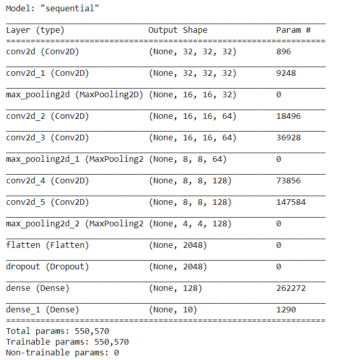
Image Source: Author

#Model -compiling
cnn_model.compile(loss="sparse_categorical_crossentropy", optimizer="Adam", metrics=["sparse_categorical_accuracy"])

#Model - training
cnn_model.fit(x_train,y_train,epochs=15)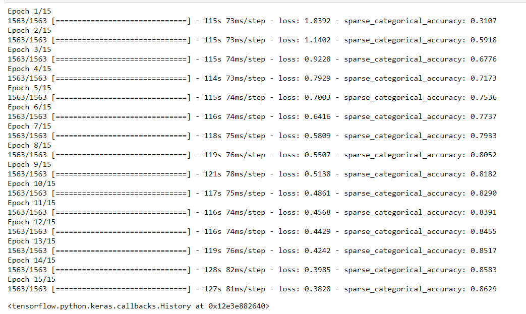

test_loss, test_accuracy = cnn_model.evaluate(x_test, y_test)

print("Test accuracy: {}".format(test_accuracy))

For full code https://github.com/anandprems/cnn

EndNote:

Did you find this article helpful? Please share your opinions/thoughts in the comments section below. Learn from mistakes is my favourite quote, if you found anything wrong too, just highlight it, I am ready to learn from the learners like you people.

About me in short, I am Premanand.S, Assistant Professor Jr and a researcher in Machine Learning. Love to teach and love to learn new things in Data Science. Mail me for any doubt or mistake, [email protected], and my Linkedin https://www.linkedin.com/in/premsanand/

FAQs