Overview

(source)
Hola Amigos!!
In this blog, we will be going through the following topics:
- Introduction to Convolutional Neural Networks and Transfer Learning.
- Face Mask Detection using a simple CNN model.
- Face Mask Detection using Transfer Learning.
Table of Contents
1. Introduction
1.1 Convolutional Neural Networks
1.2 Transfer Learning
2. Pretrained Models
2.1 Definition
2.2 Introduction to RestNet34
3. Problem Description: Face Mask Detection
4. Problem Solution
4.1 Using Convolutional Neural Networks (CNNs).
4.2 Transfer Learning using pre-trained ResNet34 model with weights.
4.3 Transfer Learning using pre-trained ResNet34 model without weights.
5. Conclusion
1. Introduction
1.1 Convolutional Neural Networks
A Convolutional Neural Network (ConvNet/CNN) is a Deep Learning system that can take in an image, assign importance (learnable weights and biases) to distinct aspects/objects in the image to discriminate one from the other. Through the use of appropriate filters, a ConvNet may successfully capture the Spatial and Temporal relationships in the image. Convolutional networks are made up of three layers: input, output, and one or more hidden layers. Convolution layers, pooling layers, normalizing layers, and fully connected layers make up the hidden layers. A convolutional network differs from a standard neural network in that its layers’ neurons are arranged in three dimensions (width, height, and depth dimensions).

The above figure describes how an input image of a traffic sign is filtered by 4 5*5 convolutional kernels, which provide four feature maps, which are then subsampled using max pooling. The following layer applies 10 5*5 convolutional kernels to the subsampled pictures, and the feature maps are pooled once again. The final layer is a fully linked layer that combines all created features and uses them in the classifier. (source)
1.2 Transfer Learning
Transfer learning is the process of applying a pre-trained model to a new task, i.e. transferring knowledge from one task to another. This is advantageous since the model does not have to learn from scratch and can attain higher accuracy in lesser time.

(source)
So for example, if we have got a neural network model that has been trained from scratch, putting in all the efforts required in the process, and it has learned well to classify images of different images of food, like pasta, noodles, etc. Then we can use the knowledge or part of it to create a model to classify different images of cars. Amazing Right!!
Transfer learning has become increasingly popular in the machine learning sector in recent years for the following reasons:
1. Growth of the ML community and information exchange:
Over the last several years, prominent institutions and tech businesses have increased their research and investment in machine learning, and there is a strong desire to share cutting-edge models and datasets with the community enabling people to quickly bootstrap using pre-trained models in a certain domain.
2. Another significant driver is that many difficulties have common sub-problems:
For example, much visual understanding and prediction categories, activities such as finding edges, limits, and background are common sub-problems.
3. Data and training resources for supervised learning are limited:
Many real-world applications are still mapped onto supervised learning tasks in which the model is asked to predict a label. One major issue is the scarcity of training data, which makes it difficult for models to generalize well. One significant advantage of doing transfer learning is that we can start learning from pre-trained models, allowing us to use knowledge from similar domains.
Techniques for Using Transfer Learning
1. Keep the pre-trained model’s initial layers and remove the final layers. Combine the new layer with the remaining chunk and train it for final classification.
2. Fine-tuning the existing parameters in a pre-trained network, i.e. optimizing the model parameters during training for the supervised prediction. Fine-tuning the model necessitates determining how many levels can be frozen and how many final layers must be fine-tuned. Thus an understanding of the model’s network structure and the role of each layer is essential.
2. Pretrained Models
2.1 Definition
Pre-trained models pass on their learning to new models by sharing their weights and biases matrices. As a result, anytime we perform transfer learning, we can transmit its weight and bias matrix to the new model.
2.2 Introduction to RestNet34
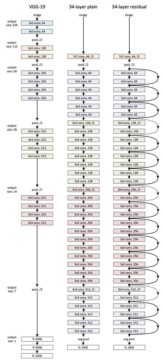
Resnet34 is one pre-trained model that is basically a 34-layer convolutional neural network that has been pre-trained using the ImageNet dataset, which contains over 100,000 images from 200 distinct classes. However, it differs from standard neural networks in that it incorporates residuals from each layer in the succeeding connected layers.
ResNet34 Architecture. (source)

3. Problem Description: Face Mask Detection
Due to global lockdowns caused by the COVID19 epidemic, wearing a face mask has just been essential for anybody venturing outside. Deep Learning Approach for Detecting Faces With and Without masks has also become a popular practice. I here attempted to train models that detect face masks on 7553 photos with three color channels (RGB).
Dataset collected from Kaggle.
4. Problem Solution
Data Exploration
import os
from torchvision.datasets import ImageFolder
from torchvision.transforms import ToTensor

data_dir = '../input/face-mask-dataset/data'
dataset = ImageFolder(data_dir, transform=ToTensor())
print(len(dataset))
print(dataset.classes)
Output–
7553
['with_mask','without_mask']
import torch
import matplotlib.pyplot as plt
%matplotlib inline

def show_example(img, label):
    print('Label: ', dataset.classes[label], "("+str(label)+")")
    plt.imshow(img.permute(1, 2, 0))

show_example(*dataset[0])
Resizing the image and cropping it to 32 * 32-pixel image, and also normalizing the pixel values to the mean and standard deviation of Imagenet images.
import torchvision.transforms as tt
image_size = (32,32)
stats = ([0.5, 0.5, 0.5], [0.5, 0.5, 0.5])
dataset = ImageFolder(data_dir, tt.Compose([
    tt.Resize(image_size),
    tt.ToTensor(),
    tt.Normalize(*stats)
]))
Creating Training and Validation Sets
from torch.utils.data import random_split
val_pct = 0.1
val_size = int(val_pct * len(dataset))

train_ds, valid_ds = random_split(dataset, [len(dataset) - val_size, val_size])
Loading the training and validation dataset to Pytorch using DataLoader
from torch.utils.data import DataLoader
batch_size = 256

train_dl = DataLoader(train_ds, batch_size, shuffle=True, num_workers=4, pin_memory=True)
valid_dl = DataLoader(valid_ds, batch_size*2, num_workers=4, pin_memory=True)

from torchvision.utils import make_grid
def denormalize(images, means, stds):
    if len(images.shape) == 3:
        images = images.unsqueeze(0)
    means = torch.tensor(means).reshape(1, 3, 1, 1)
    stds = torch.tensor(stds).reshape(1, 3, 1, 1)
    return images * stds + means

def show_image(img_tensor, label):
    print('Label:', dataset.classes[label], '(' + str(label) + ')')
    img_tensor = denormalize(img_tensor, *stats)[0].permute((1, 2, 0))
    plt.imshow(img_tensor)

def show_batch(dl):
    for images, labels in dl:
        fig, ax = plt.subplots(figsize=(16, 16))
        ax.set_xticks([]); ax.set_yticks([])
        images = denormalize(images[:64], *stats)
        ax.imshow(make_grid(images, nrow=8).permute(1, 2, 0))
        break
show_batch(train_dl)
Defining Image Classification base class
import torch.nn as nn
import torch.nn.functional as F

def accuracy(outputs, labels):
    _, preds = torch.max(outputs, dim=1)
    return torch.tensor(torch.sum(preds == labels).item() / len(preds))

class ImageClassificationBase(nn.Module):
    def training_step(self, batch):
        images, labels = batch
        out = self(images)                  # Generate predictions
        loss = F.cross_entropy(out, labels)  # Calculate loss
        return loss

    def validation_step(self, batch):
        images, labels = batch
        out = self(images)                    # Generate predictions
        loss = F.cross_entropy(out, labels)   # Calculate loss
        acc = accuracy(out, labels)           # Calculate accuracy
        return {'val_loss': loss.detach(), 'val_acc': acc}

    def validation_epoch_end(self, outputs):
        batch_losses = [x['val_loss'] for x in outputs]
        epoch_loss = torch.stack(batch_losses).mean()   # Combine losses
        batch_accs = [x['val_acc'] for x in outputs]
        epoch_acc = torch.stack(batch_accs).mean()      # Combine accuracies
        return {'val_loss': epoch_loss.item(), 'val_acc': epoch_acc.item()}

    def epoch_end(self, epoch, result):
        print("Epoch [{}],{} train_loss: {:.4f}, val_loss: {:.4f}, val_acc: {:.4f}".format(
            epoch, "last_lr: {:.5f},".format(result['lrs'][-1]) if 'lrs' in result else '',
            result['train_loss'], result['val_loss'], result['val_acc']))
Defining Evaluation Functions
import torch
from tqdm.notebook import tqdm

@torch.no_grad()
def evaluate(model, val_loader):
    model.eval()
    outputs = [model.validation_step(batch) for batch in val_loader]
    return model.validation_epoch_end(outputs)

def fit(epochs, lr, model, train_loader, val_loader, opt_func=torch.optim.SGD):
    history = []
    optimizer = opt_func(model.parameters(), lr)
    for epoch in range(epochs):
        # Training Phase
        model.train()
        train_losses = []
        for batch in tqdm(train_loader):
            loss = model.training_step(batch)
            train_losses.append(loss)
            loss.backward()
            optimizer.step()
            optimizer.zero_grad()
        # Validation phase
        result = evaluate(model, val_loader)
        result['train_loss'] = torch.stack(train_losses).mean().item()
        model.epoch_end(epoch, result)
        history.append(result)
    return history

def get_lr(optimizer):
    for param_group in optimizer.param_groups:
        return param_group['lr']

def fit_one_cycle(epochs, max_lr, model, train_loader, val_loader,
                  weight_decay=0, grad_clip=None, opt_func=torch.optim.SGD):
    torch.cuda.empty_cache()
    history = []

    # Set up custom optimizer with weight decay
    optimizer = opt_func(model.parameters(), max_lr, weight_decay=weight_decay)
    # Set up one-cycle learning rate scheduler
    sched = torch.optim.lr_scheduler.OneCycleLR(optimizer, max_lr, epochs=epochs,
                                                steps_per_epoch=len(train_loader))

    for epoch in range(epochs):
        # Training Phase
        model.train()
        train_losses = []
        lrs = []
        for batch in tqdm(train_loader):
            loss = model.training_step(batch)
            train_losses.append(loss)
            loss.backward()

            # Gradient clipping
            if grad_clip:
                nn.utils.clip_grad_value_(model.parameters(), grad_clip)
            optimizer.step()
            optimizer.zero_grad()

            # Record & update learning rate
            lrs.append(get_lr(optimizer))
            sched.step()
        # Validation phase
        result = evaluate(model, val_loader)
        result['train_loss'] = torch.stack(train_losses).mean().item()
        result['lrs'] = lrs
        model.epoch_end(epoch, result)
        history.append(result)
    return history
4.1 Using Convolutional Neural Networks (CNNs)
class CnnModel(ImageClassificationBase):
    def __init__(self):
        super().__init__()
        self.network = nn.Sequential(
            # input: 3*32*32
            nn.Conv2d(3, 32, kernel_size=3, padding=1),
            # output: 32*32*32
            nn.ReLU(),
            # output: 32*32*32
            nn.Conv2d(32, 64, kernel_size=3, stride=1, padding=1),
            # output: 64*32*32
            nn.ReLU(),
            # output: 64*32*32
            nn.MaxPool2d(2, 2), # output: 64 x 16 x 16
            nn.Conv2d(64, 128, kernel_size=3, stride=1, padding=1),
            nn.ReLU(),
            nn.Conv2d(128, 128, kernel_size=3, stride=1, padding=1),
            nn.ReLU(),
            nn.MaxPool2d(2, 2), # output: 128 x 8 x 8
            nn.Conv2d(128, 256, kernel_size=3, stride=1, padding=1),
            nn.ReLU(),
            nn.Conv2d(256, 256, kernel_size=3, stride=1, padding=1),
            nn.ReLU(),
            nn.MaxPool2d(2, 2), # output: 256 x 4 x 4
            nn.Flatten(), #flatten to vector of class 10
            nn.Linear(256*4*4, 1024),
            nn.ReLU(),
            nn.Linear(1024, 512),
            nn.ReLU(),
            nn.Linear(512, 10))

    def forward(self, xb):
        return self.network(xb)

model = to_device(CnnModel(), device)
model

4.2 Transfer Learning using pre-trained ResNet34 model with weights from pre-training on Imagnet dataset.
Defining MasksModel class for mask/without mask image classification using pre-trained model Restnet34
from torchvision import models
models.resnet34(pretrained=True)


class MasksModel(ImageClassificationBase):

    def __init__(self, num_classes, pretrained=True):
        super().__init__()
        # Use a pretrained model
        self.network = models.resnet34(pretrained=pretrained) #downloading weights from this model when it was trained on ImageNet dataset
        # Replace last layer
        self.network.fc = nn.Linear(self.network.fc.in_features, num_classes)

    def forward(self, xb):
        return self.network(xb)

model = MasksModel(len(dataset.classes), pretrained=True)
to_device(model, device);

%%time
history += fit_one_cycle(epochs, max_lr, model, train_dl, valid_dl,
                         grad_clip=grad_clip,
                         weight_decay=weight_decay,
                         opt_func=opt_func)
4.3 Transfer Learning using pre-trained ResNet34 model without weights.
model2 = MasksModel(len(dataset.classes), pretrained=False)
to_device(model2, device);

%%time
history2 += fit_one_cycle(epochs, max_lr, model2, train_dl, valid_dl,
                         grad_clip=grad_clip,
                         weight_decay=weight_decay,
                         opt_func=opt_func)

5. Conclusion
| Model | Training Loss | Validation Loss | Validation Accuracy |
| Convolutional Neural Network | 0.27 | 0.26 | 0.88 |
| ResNet34 with weights | 0.009 | 0.06 | 0.97 |
| ResNet34 without weights | 0.03 | 0.10 | 0.96 |
From the above table, we can conclude that our model had learned much much better when we used transfer learning through the pre-trained ResNet34 model with weights. Also, if we compare the two transfer learning processes, one with weights and the other without weights, we can see that there is a significant difference between the training and validation loss, hence indication a possibility of overfitting which is very well handled when using ResNet34 with the weights assigned from it pre-training on Imagenet dataset.
The media shown in this article are not owned by Analytics Vidhya and are used at the Author’s discretion.


