Know About Apache Spark Using PySpark for Data Engineering

This article was published as a part of the Data Science Blogathon

Introduction-

In this article, we will explore Apache Spark and PySpark, a Python API for Spark. We will understand its key features/differences and the advantages that it offers while working with Big Data. Later in the article, we will also perform some preliminary Data Profiling using PySpark to understand its syntax and semantics.

Key features of PySpark-

Distributed Computing-

To understand why distributed computing is required for processing large workloads, it is essential for us to first know what Big Data is. Big Data is commonly used to refer to data that is so large that it is very difficult to deal with using traditional tools and methods. (The largeness of data is identified in the form of 3 V’s: Volume of data, Velocity of incoming data streams, Variety of data – i.e structured, unstructured, and semistructured)

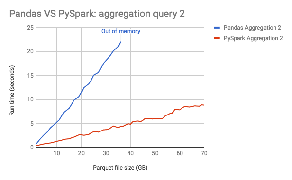
As you can infer from the graph below, Pandas (A Python library for operating on tabular data, used extensively by the Data Science community) performs operations much faster than PySpark when the size of data is small. However as the size increases, PySpark starts performing better than Pandas, and there is a tipping point after which Pandas is unable to operate upon the large data. We will understand why Pandas ran “out of memory” and how Spark mitigates through this problem. 

Pandas operates on data by loading the data as a whole into the memory of the machine. So if the device that you are using has a memory of 32 GB, the performance of Pandas will deteriorate as your data size approaches 32 GB and you will have less memory for other things on your computer. It will run out of memory once you exceed 32 GB since it cannot load the entire block as a whole within the available memory.

Spark overcomes this problem by using a network of machines/nodes known as clusters. So a large task is divided into several subtasks and these subtasks are assigned to individual nodes. The nodes carry out the subtasks and the individual output of each node is aggregated to achieve the final output.

Let us understand this by a simple analogy – Let’s say you and your friend have been challenged by your maths teacher to solve 10 addition operations within a minute. In the first attempt, both you and your friend started adding and both of you were able to add the first 6 numbers only before you ran out of time. ( 6 numbers added in 60 seconds = 1 in 10 seconds for simplicity). So for the second attempt, you devise a new strategy. While your friend starts adding the numbers from the beginning, you start adding numbers from the end. At the end of 50 seconds, your friend has found the sum of the first 5 numbers and you have found the sum of the last 5 numbers. In the last 10 seconds, you add the two sums and find the sum of all ten numbers, thus impressing your maths teacher.

In-memory- 

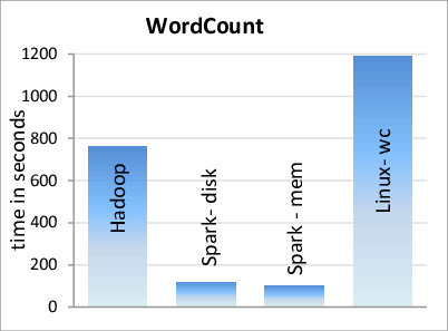
Spark is said to be lightning-fast for large-scale data processing. This is because it saves and loads data from distributed memory (RAM) over a cluster of machines. RAM has a much higher processing speed than Hard drives. When the data does not fit into RAM, it is either recalculated or spilled to Hard drives. Spark can process data up to 100 times faster than Hadoop when the data is stored entirely in memory and up to 10 times faster when some of the data is spilled onto Hard drives.

 

Immutability-

Immutability in PySpark essentially means that when we try to apply changes to an object, instead of modifying the object, we create a new object reference. Immutability along with DAG (Directed Acyclic Graph, explained later) helps Spark with fault tolerance which gives it the ability to recover from the loss in case of failure. (The syntax to interact with immutable objects varies a little and is explained later in the article along with code and examples)

Lazy evaluation-

Spark supports two types of operations – TRANSFORMATIONS and ACTIONS.

Transformations are functions that take an object as the input and produce one or many objects as output. They do not change the input object. Actions are operations performed on objects that perform the computation and send the results back to the driver.

Lazy evaluation means that Transformations applied on an object are not executed till an Action is triggered. When an Action is triggered, Spark creates a DAG (Directed Acyclic Graph) of all the operations that need to be performed and finds the best path to perform the required operations, thus saving resources and providing optimum results.

This can be understood with the help of an analogy. Let’s say your maths teacher, who also happens to be your class teacher, wants to know if Jim, a student in the class adjacent to you, is present or not. You go to the adjacent class and enquire if Jim is present. Your teacher also wanted to know if Pam, a student in the same class, was present or not. You go to the adjacent class again and ask if Pam is present. Let’s say the same process happens a few more times as he wishes to know about Michael, Dwight, and Jan’s attendance. Instead of immediately going to the adjacent class to perform the given task, you could have waited for a list of all the students whose attendance is to be known, thus saving a lot of time and resources.

The features discussed above make Spark scalable, fast, resilient, and optimum when it comes to working with Big Data. We will now learn the basic syntax and semantics of PySpark and perform Data Profiling on a sample dataset.

Data Profiling using Pyspark

iris_df = spark.read.csv('dbfs:/FileStore/shared_uploads/[email protected]/irisdataset.csv' , header = "true" , inferSchema = "true")

In the spark.load.csv function, we pass 3 arguments which are the filepath, header (which is kept true if our file contains the names of the columns in the first/header line, as in our case), and infer schema (which is kept true in order to infer datatypes of columns automatically, instead of assigning the default string values)

iris_df.show()

The show function prints the rows of the dataframe to the console. We can pass an optional parameter to select the number of rows to be displayed.

iris_df.show(5)

iris_df.columns

The columns function returns all the columns of the dataframe as a list.

iris_df.dtypes

The dtypes function returns all column names with their respective datatypes as a list.

iris_df.describe().show()

The describe function computes basic statistical values such as count, mean, standard deviation, minimum and maximum value for all columns having numeric and string datatype values.

iris_df[iris_df.sepal_length > 3].show()

We can filter a part of the dataframe by passing a condition having a boolean value in square brackets. The above command displays all rows in the dataframe having sepal length greater than 3.

The following commands are used to perform aggregation functions on grouped column values

iris_df.groupby('species').count().show()

The above command displays the number/frequency of values of each type of species.

iris_df.groupby('species').mean('sepal_length').show()

The above command displays the mean sepal length value for each type of species.

iris_df.groupby('species').mean('sepal_length','petal_length').show()

The above command displays a list containing the mean sepal length and petal length values for each type of species.

Window Functions – PySpark Window functions process a group of rows like a frame or partition and return a single value for every input row.

In the below function we have created partitions based on species and then calculated the average, sum, minimum and maximum values for the sepal length column. The same can be applied to any other column as well.

windowSpecAgg  = Window.partitionBy("species")
from pyspark.sql.functions import col,avg,sum,min,max,row_number 
iris_df.withColumn("row",row_number().over(windowSpec)) 
  .withColumn("avg", avg(col("sepal_length")).over(windowSpecAgg)) 
  .withColumn("sum", sum(col("sepal_length")).over(windowSpecAgg)) 
  .withColumn("min", min(col("sepal_length")).over(windowSpecAgg)) 
  .withColumn("max", max(col("sepal_length")).over(windowSpecAgg)) 
  .where(col("row")==1).select("species","avg","sum","min","max") 
  .show()

Conclusion and Scope for further reading-

In this article, I have tried to deliver the key features and advantages of using Spark concisely. The basic Data Profiling tutorial in the latter part of the article was to acquaint the reader with the syntax of PySpark. PySpark supports a large number of useful modules and functions, discussing which are beyond the scope of this article. Hence I have attached the link to the official Spark and PySpark documentation which intrigued readers can use for further reading.

https://spark.apache.org/docs/latest/quick-start.html

Hope you liked the article!

The media shown in this article are not owned by Analytics Vidhya and are used at the Author’s discretion.