Understanding Sequential Vs Functional API in Keras

This article was published as a part of the Data Science Blogathon

Introduction

Neural networks play an important role in machine learning. Inspired by how human brains work, these computational systems learn a relationship between complex and often non-linear inputs and outputs. A basic neural network consists of an input layer, a hidden layer and an output layer. Each layer is made of a certain number of nodes or neurons. Neural networks with many layers are referred to as deep learning systems.

Neural networks are very complex in architecture and computationally expensive.

Luckily we have Keras, a deep learning API written in Python running on top of Tensorflow, that makes our work of building complex neural networks much easier.

Keras offers two ways to build neural networks. They are as follows:

          1.using Sequential API

Here we create the model layer-by-layer. It is very simple and easy to use. But sharing of layers or branching of layers is not allowed (We will see what sharing or branching means later). Also, you can’t have multiple inputs or outputs.

          2.using Functional API

It is more flexible than the sequential API. It is more powerful than the sequential API in the sense branching or sharing of layers is allowed here. And also it can have multiple inputs and outputs.

So which one to use? In this article, we will try to understand the two different architectures and which one to use when.

We will use a toy neural network for better understanding and visualization and then will try to understand using the codes and apply it to a real use case.

We will focus more on the functional API as it is helpful to build more complex models.

TOY neural network 

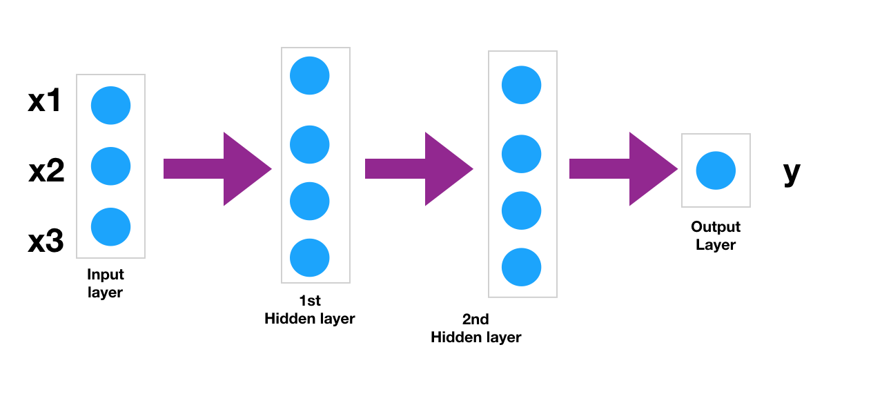
Let’s say we want to build a neural network that has 3 inputs (x1,x2,x3), 2 hidden layers with 4 neurons each and one output y.

This is how it looks like.

Now let’s proceed to build the neural network using both the APIs for the above network

A.Using Sequential API  

##Import the libraries

from tensorflow.keras.models import Sequential
from tensorflow.keras.layers import Dense, Activation
from tensorflow.keras.optimizers import Adam

## Creating the model

model = Sequential()

model.add(Dense(4,activation='relu')) ##<----- You don't have to specify input size.Just define the hidden layers 
model.add(Dense(4,activation='relu'))
model.add(Dense(1))

## defining the optimiser and loss function
model.compile(optimizer='adam',loss='mse')

## training the model
model.fit(x=X_train,y=y_train,
          validation_data=(X_test,y_test),
          batch_size=128,epochs=400)

Notice :
You don’t have to specify a separate input layer in the sequential API. It automatically recognizes the input shape.

B.Using Functional API  

• Here you define an input layer and specify the input size= Input(shape=)

• You define a layer by giving it a name, specifying the number of neurons, activation function, etc.
• Then put the previous layer in a set of parentheses.

 = Dense(, activation=)()

The code below will give you better clarity.

##Import the libraries
from tensorflow.keras.models import Model
from tensorflow.keras.layers import Input,Dense

## Creating the layers
input_layer = Input(shape=(3,))
Layer_1 = Dense(4, activation="relu")(input_layer)
Layer_2 = Dense(4, activation="relu")(Layer_1)
output_layer= Dense(1, activation="linear")(Layer_2)
##Defining the model by specifying the input and output layers
model = Model(inputs=input_layer, outputs=output_layer)
## defining the optimiser and loss function
model.compile(optimizer='adam',
              loss='mse')
## training the model
model.fit(X_train, y_train,epochs=400, batch_size=128,validation_data=(X_test,y_test))

Because you can define any layer separately and independently the functional API enables us for branching and multiple inputs and outputs.
What it means is you can branch out and add one (or any number of) different layers from any layer.

The following image explains branching and multiple outputs.

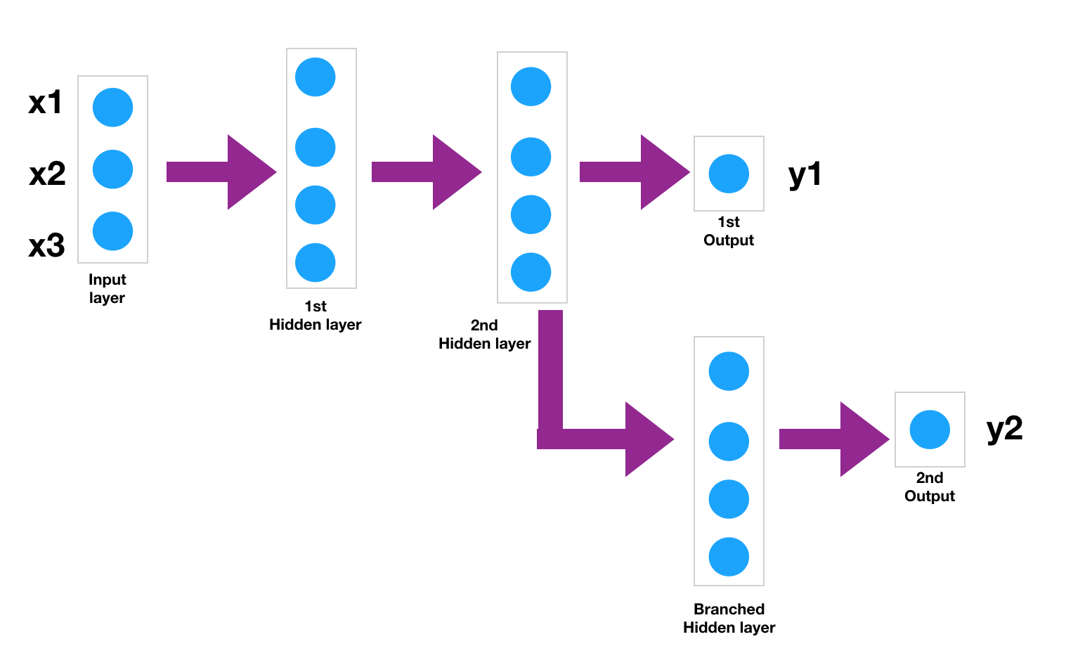
As it is evident one more layer is added after the 2nd hidden layer. The output of the 2nd hidden layer is used to predict ‘y1’ and at the same time is fed to one more layer(Branched hidden layer)which predicts a 2nd output ‘y2’.

You can add more layers and more neurons for predicting the 2nd output. This is where the functional API wins over the sequential API, because of the flexibility it offers. Using this we can predict multiple outputs at the same time. We would have built 2 different neural networks to predict outputs y1 and y2 using sequential API  but the functional API enabled us to predict two outputs in a single network.

Use case(Predicting Energy output and exhaust vacuum for a Power Plant) 

Let’s apply the functional API to real-world data. We are going to use the combined cycle power plant data set from the UCI machine learning repository. Download the dataset from the below link.

https://archive.ics.uci.edu/ml/datasets/Combined+Cycle+Power+Plant

Dataset information(Taken from above link):

The dataset contains 9568 data points collected from a Combined Cycle Power Plant over 6 years (2006-2011) when the power plant was set to work with a full load.
A combined-cycle power plant (CCPP) is composed of gas turbines (GT), steam turbines (ST) and heat recovery steam generators. In a CCPP, the electricity is generated by gas and steam turbines, which are combined in one cycle, and is transferred from one turbine to another. While the Vacuum is collected from and has an effect on the Steam Turbine, the other three of the ambient variables affect the GT performance.

Attribute Information(Taken from above link):

Features consist of hourly average ambient variables
– Temperature (T) in the range 1.81°C and 37.11°C.
– Ambient Pressure (AP) in the range 992.89-1033.30 millibar.

– Relative Humidity (RH) in the range 25.56% to 100.16%.
– Exhaust Vacuum (V) in the range 25.36-81.56 cm Hg.
– Net hourly electrical energy output (PE) 420.26-495.76 MW.

Let’s build a neural network using functional API to predict Net hourly electrical energy output (PE) and Exhaust Vacuum (V) with Temperature (T), Ambient Pressure (AP) and Relative Humidity (RH) as inputs.

##import libraries
import numpy as np
import pandas as pd
import tensorflow as tf
from sklearn.model_selection import train_test_split
from sklearn.preprocessing import MinMaxScaler
import matplotlib.pyplot as plt

##import the dataset 

df = pd.read_excel('Folds5x2_pp.xlsx')

df.head()

##define a function to get the outputs of the model

def get_outputs(data):

y1 = data.pop('PE')

y1 = np.array(y1)

y2 = data.pop('V')

y2 = np.array(y2)

return y1, y2

# Split the data into train and test with 80 train / 20 test

train, test = train_test_split(df, test_size=0.2, random_state = 1)




##getting the outputs(PE) and (V) of the train and test data 

y_train = get_outputs(train)

y_test = get_outputs(test)

###Scaling the inputs

min_max=MinMaxScaler()

X_train=min_max.fit_transform(train)

X_test=min_max.transform(test)

##Import the libraries for neural networks

from tensorflow.keras.models import Model

from tensorflow.keras.layers import Input

from tensorflow.keras.layers import Dense

Building the neural network

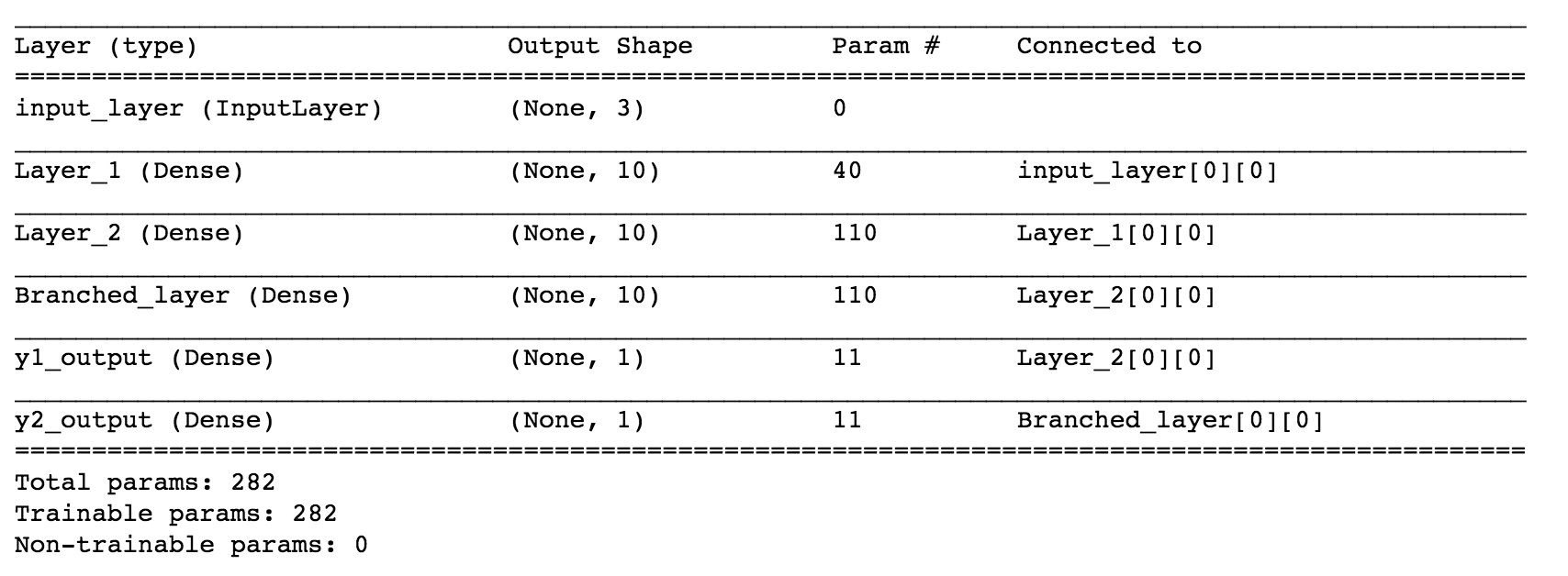
(Here we are using 2 hidden layers and one branched layer with 10 neurons each)

##define input layer

input_layer = Input(shape=(3,),name='input_layer')

##Defining 2 hidden layers

Layer_1 = Dense(10, activation="relu",name='Layer_1')(input_layer)

Layer_2 = Dense(10, activation="relu",name='Layer_2')(Layer_1)

##Defining  output layer y1

y1_output= Dense(1, activation="linear",name='y1_output')(Layer_2)

##Defining Branched layer

Branched_layer=Dense(10, activation="relu",name='Branched_layer')(Layer_2)

##Defining 2nd output layer y2

y2_output= Dense(1, activation="linear",name='y2_output')(Branched_layer)

##Defining the model by specifying the input and output layers

model = Model(inputs=input_layer,outputs=[y1_output,y2_output])

## defining the optimiser and loss function

model.compile(optimizer='adam',

              loss={'y1_output':'mse','y2_output':'mse'})

##training the model

model.fit(X_train,y_train,

               epochs=1000, batch_size=128, validation_data=(X_test,y_test))

##model predictions

predictions = model.predict(X_test)

predicted_energy=predictions[0]

predicted_vacuum=predictions[1]

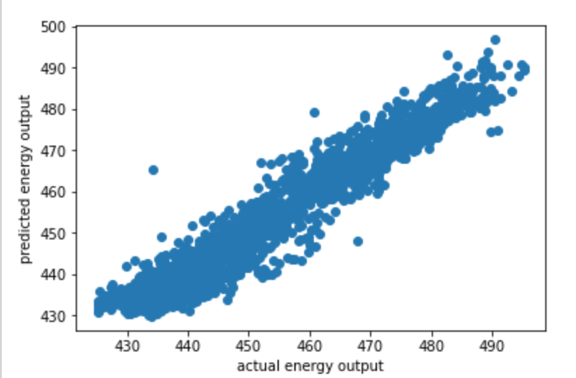
##Plotting actual vs predicted energy

plt.scatter(y_test[0],predicted_energy)

plt.xlabel('actual energy output')

plt.ylabel('predicted energy output')

##Plotting actual vs predicted exhaust vacuum

plt.scatter(y_test[1],predicted_vacuum)

plt.xlabel('actual exhaust vacuum')

plt.ylabel('predicted exhaust vacuum')

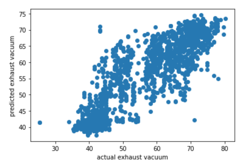
Looks like our model is doing better in predicting the energy output than predicting the exhaust vacuum.

Checking r2 score:

print('r2 score for energy predicted :',r2_score(y_test[0],predicted_energy))

print('r2 score forexhaust vacuum predicted :',r2_score(y_test[1],predicted_vacuum))

The predictions can be further improved by tuning various hyperparameters.

Conclusion:

• The functional API offers more flexibility and control over the layers than the sequential API.
• It can be used to predict multiple outputs(i.e output layers) with multiple inputs(i.e input layers))

Thank you for reading!

Feel free to leave a comment below.

The media shown in this article are not owned by Analytics Vidhya and are used at the Author’s discretion.