This article was published as a part of the Data Science Blogathon
Introduction
In our previous article, we have discussed Logistic Regression, and later in the code section, we have used “Gradient Descent“ and “Stochastic Gradient Descent”. In this article, we will discuss gradient descent.
Gradient descent is an optimization algorithm used to optimize neural networks and many other machine learning algorithms. Our main goal in optimization is to find the local minima, and gradient descent helps us to take repeated steps in the direction opposite of the gradient of the function at the current point.
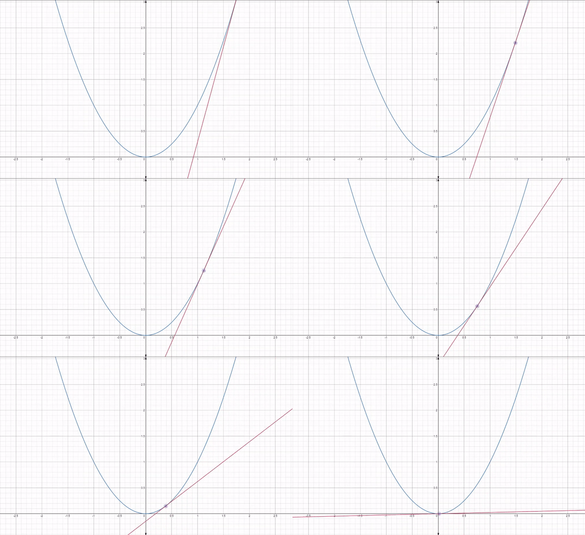
Fig 1: How gradient descent works
Table of Contents
- Random initialization(guesswork)
- Geometric intuition of Gradient Descent
- What is the Learning rate?
- Code
- Conclusion
Random initialization
Suppose we have a model f(x)= 1/(1+exp(-wx+b))
Loss function L(w,b) = (yi-f(x))2 and we will try to find the parameters which minimizes the loss.
To simplify the process further we will consider that the model has only one input w1 and b(bias)
Now let us manually find the optimal w*, b* and we are assuming that we don’t have any proper technique to find these values. So let’s randomly guess the initial values of w and b
w=0.5 and b = 0
Now, let us train our model with only two data points
|
|
|
|
| 0.5 | 0 | [(2.5,0.9),(0.5,0.2)] | 0.073 |
Our loss L(w,b) is not close enough to 0, so let’s continue guessing more w’s and b’s until we find the values which are close enough to 0.
| w | b | L(w,b) |
| 0.50 | 0.00 | 0.0730 |
| -0.10 | 0.00 | 0.1481 |
| 0.94 | -0.94 | 0.0028 |
| 1.42 | -1.73 | 0.0028 |
| 1.65 | -2.08 | 0.0003 |
| 1.78 | -2.27 | 0.0000 |
If you notice our the loss of our second guess is greater than the first guess due to the negative input in w. In our third guess, we input negative values for the bias term which reduces the loss than the first one. So, we keep on randomly guessing the values based on the observation of the loss. Even though our random guesswork is driven by the loss function still this is a pure brute force approach.
Now with the increase in the number of parameters and the number of data points we can not stick to any brute force techniques. We need to have a more effective, principled approach so that we can reach the minimum value of the error surface.
Geometric Intuition of Gradient Descent
A gradient simply measures the change in all the weights(dw) concerning the change in error(dL). So the process is iterative as we first randomly guess our values(considering we have only a single input w and bias b) then we calculate the loss for each iteration and using the Gradient Descent algorithm we move on to the 2nd iteration, then 3rd, 4th, …. kth until our loss converges.
.png)
Fig 2: Slope changing its sign from positive to negative
Initially when we randomly guess the value of our parameters(w and b). Gradient descent then starts at the point either on the positive or on the negative side(around the top). Then it takes one step after another in the steepest downside direction(from the top to the bottom). As our main goal is to reach the local minima we continue until it reaches where the loss is as small as possible.
Let’s understand stepwise:
1) Pick a random weight witeration_0 initially.
2) Now we want to pick the witeration_1 such that the loss(witeration_1) must be less than loss(witeration_0).
Therefore we will use the gradient descent equation: wnew = wold – eta*(dL/dw)old
For example:
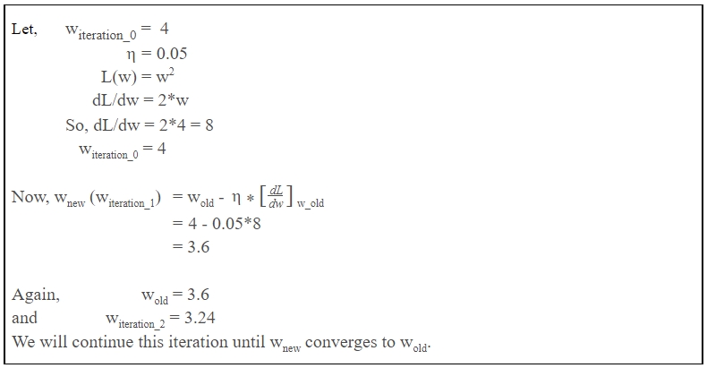
We have got an idea of how gradient descent works. So lets look into the derivative((dL/dw)) part in the equation.
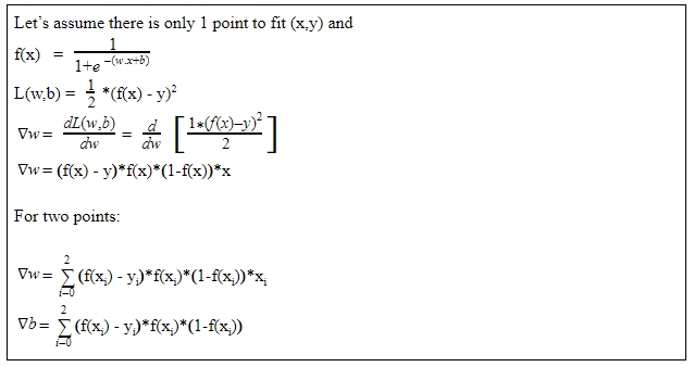
Now our equation becomes:

Learning Rate
The whole idea of gradient descent is to optimize the approach of reaching the local minima and we may take big steps to take gradient descent into the direction of local minimum or we may want to be more conservative, moving only by a small amount, these steps sizes are determined by learning rate i.e. “eta“
Case 1: Bounce back between the convex function and not reaching the local minimum
Let us take one example:
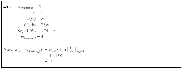
Since we want to take a big step so we set the value of eta = 1
As a result we got witeration_0 = 4 , witeration_1 = -4, witeration_2 = 4
Because the steps size being too big, it simply jumping back and forth between the convex function of gradient descent. In our case even if we continue till ith iteration we will not reach the local minima.
.gif)
Fig 3: Bounce back between the convex function and not reaching the local minimum(learning rate=1)
Case 2: Bounce back between the convex function and reaching the local minimum
In this example we are considering learning rate(eta) = 0.9. In this case, initially, it bounces back and forth between the convex function but after several iterations, it reaches the local minima.
.gif)
Fig 4: Bounce back between the convex function and not reaching the local minimum(learning rate=0.9)
Case 3: Very small learning rate
Lets us again take an example where we consider moving only by a small step. So we set the value of eta = 0.05
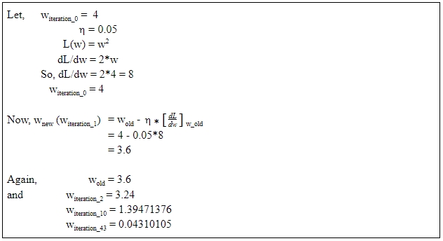
Here in this example, we slowly move toward the local minima after each iteration and eventually reach the local minimum after 30 iterations. So to optimize this process we must not choose a very low learning rate.
.gif)
Fig 5: Conservative learning rate
Case 4: Optimal learning rate
The learning rate should never be too big nor too small because a very small learning rate will eventually reach the local minima but that may take a while. In this case, we are considering our learning rate = 0.35 which reaches the local minima faster in less than 15 iterations.
.gif)
Fig 6: Optimal learning rate
Our main goal is to reach similar results with fewer steps.
Understanding the Code
The code is very straightforward, you can try tweaking the learning rate and plot the error surface.
X = [0.5, 2.5]

Y = [0.2, 0.9]

# Sigmoid function with parameters w,b

def f(w,b,x):

	return 1.0/(1.0+np.exp(-(w*x + b)))

# We are using Mean Sq. Loss

def error (w, b):

	error = 0.0

	for x,y in zip(X, Y):

		fx = f(w, b, x)

		err += 0.5 * (fx - y) **2

	return err

#Calculating the gradients

def grad_b(w,b,x,y):

	fx = f(w,b,x)

	return (fx-y)*fx*(1-fx)

def grad_w(w,b,x,y):

	fx = f(w,b,x)

	return (fx-y)*fx*(1-fx)*x

#Main loop

def do_gradient_descent():

	w, b, eta, max_epochs = -2, -2, 0.3, 1000

	for i in range(max_epochs):

		dw, db = 0, 0

		for x,y in zip(X, Y):

			dw += grad_w(w, b, x, y)

			db += grad_b(w, b, x, y)

		w = w - eta*dw

		b = b - eta*db
Conclusion
It’s important to note is that the gradient descent goes through the whole dataset for each iteration which is computationally expensive and a slow process. Also if the learning rate is too fast, it will skip the true local minima to optimize for time and if it is too slow then it may never converge because it trying really hard to exactly find a local minimum.
To deal with these issues there are variations of gradient descent used in modern machine learning and deep learning algorithms. The main focus for these variations is computational efficiency as calculating the gradient over a dataset which have millions and billions of data points is computationally expensive.
In our next article, we will briefly look into its variations and will discuss the pros and cons of each variation.


