An Introduction to Data Analysis using Spark SQL

This article was published as a part of the Data Science Blogathon

Introduction

Spark is an analytics engine that is used by data scientists all over the world for Big Data Processing. It is built on top of Hadoop and can process batch as well as streaming data. Hadoop is a framework for distributed computing that splits the data across multiple nodes in a cluster and then uses of-the-self computing resources for computing the data in parallel. As this is open-source software and it works lightning fast, it is broadly used for big data processing.

Before start, I assume that you have a certain amount of familiarity with spark, and you have worked on small applications to handle big data. Also, familiarity with Spark RDDs, Spark DataFrame, and a basic understanding of relational databases and SQL will help to proceed further in this article.

Spark Catalyst optimizer

We shall start this article by understanding the catalyst optimizer in spark 2 and see how it creates logical and physical plans to process the data in parallel.

Spark 2 includes the catalyst optimizer to provide lightning-fast execution. The catalyst optimizer is an optimization engine that powers the spark SQL and the DataFrame API.

The input to the catalyst optimizer can either be a SQL query or the DataFrame API methods that need to be processed. These are known as input relations. Since the result of a SQL query is a spark DataFrame we can consider both as similar. Using these inputs, the catalyst optimizer comes up with a logical optimization plan. But, at this stage, the logical plan is said to be unresolved because it doesn’t take into account the types of columns. In fact, at this stage, the optimizer is not aware of the existence of the columns.

This is where Catalog comes into the picture. The Catalog contains the details about every table from all the data sources in the form of a catalog. The Catalog is used to perform the analysis of the inputs and results of the logical plan.

After this point, actual optimization takes place. This is where the input will be passed to look for possible optimizations. These steps may include pruning of projections and simplifying expressions to simplify the query so that it executes more efficiently. Then the optimizer will come up with different optimizations in different combinations and will generate a collection of logical plans.

Following that, the cost of each of the plans will be calculated. The logical plan with the lowest cost in terms of resources and execution time will be picked. After the logical plan has been picked, it needs to be translated into the physical plan by taking into account the available resources. So, the lowest cost logical plan as input, number of physical plans will be generated and the cost for each of these will be calculated using the Tungsten engine. The cost calculation involves several parameters including the resource available and the overall performance and the efficiency of resource use for each of the physical plans. The output of this stage will be a Java bytecode that will run on the Sparks execution engine. This is the final output of the catalyst optimizer.

Following diagram of a high-level logical overview of catalyst optimizer:

Introduction to Spark SQL

There are several operations that can be performed on the Spark DataFrame using DataFrame APIs. It allows us to perform various transformations using various rows and columns from the Spark DataFrame. We can also perform aggregation and windowing operations.
Those who have a background working with relational databases and SQL will find the familiarity of DataFrame with relational tables. You can perform several analytical tasks by writing queries in spark SQL.

I will show several examples by which you can understand how we can treat a spark DataFrameas as a relational database table.

Creating Spark Session

For this, we need to set up the spark in our system and after we log into the Spark console, the following packages need to be imported to perform the examples.

from pyspark.sql import SparkSession
from pyspark.sql.types import *
from pyspark.sql.functions import *
from pyspark.sql.types import Row
from datetime import datetime

After the necessary imports, we have to initialize the spark session by the following command:

spark = SparkSession.builder.appName("Python Spark SQL basic example").config("spark.some.config.option", "some-value").getOrCreate()

Then we will create a Spark RDD using the parallelize function. This RDD contains two rows for two students and the values are self-explanatory.

student_records = sc.parallelize([Row(roll_no=1,name='John Doe',passed=True,marks={'Math':89,'Physics':87,'Chemistry':81},sports =['chess','football'], DoB=datetime(2012,5,1,13,1,5)), Row(roll_no=2,name='John Smith',passed=False,marks={'Math':29,'Physics':31,'Chemistry':36}, sports =['volleyball','tabletennis'], DoB=datetime(2012,5,12,14,2,5))])

Creating DataFrame

Let’s create a DataFrame from this RDD and show the resulting DataFrame by following the command.

student_records_df  = student_records.toDF()
student_records_df.show()

Now, as we can see the content of column ‘marks’ has been truncated. To view the full content we can run the following command:

student_records_df.show(truncate=False)

Creating Temporary View

The above DataFrame can be treated as a relational table. For that, by using the following command we can create a relational view named ‘records’ which is valid for the created spark session.

student_records_df.createOrReplaceTempView('records')

It is time for us to now run a SQL query against this view and show the results.

spark.sql("SELECT * FROM records").show()

Here we can verify that the spark.sql returns Spark DataFrame.

Accessing Elements of List or Dictionary within DataFrame

While creating the RDD, we have populated the ‘marks’ filed with a dictionary data structure and the ‘sports’ filed with a list data structure. We can write SQL queries that will pick specific elements from that dictionary and list.

spark.sql('SELECT roll_no, marks["Physics"], sports[1] FROM records').show()

We can specify the position of the element in the list or the case of the dictionary, we access the element using its key.

Where Clause

Let’s see the use of the where clause in the following example:

spark.sql("SELECT * FROM records where passed = True").show()

In the above example, we have selected the row for which the ‘passed’ column has the boolean value True.

We can write where clause using the values from the data structure field also. In the following example, we are using the key ‘Chemistry’ from the marks dictionary.

spark.sql('SELECT * FROM records WHERE marks["Chemistry"] < 40').show()

Creating Global View

The view ‘records’ we have created above has the scope only for the current session. Once the session disappears, the view will be terminated, and it will not be accessible. However, if we want other sessions which were initiated in the same application to be able to access the view even if the session that created the view ends, then we make a global view by using the following command:

student_records_df.createGlobalTempView('global_record')

The scope of this view will be at the application level rather than the session-level. Now, let’s run a select query on this global view:

spark.sql("SELECT * FROM global_temp.global_records").show()

All the global views are preserved in the database called: global_temp.

Dropping Columns from DataFrame

If we want to see only the columns of our DataFrame, we can use the following command:

student_records_df.columns

If we want to drop any column, then we can use the drop command. In our dataset, let’s try to drop the ‘passed’ column.

student_records_df = student_records_df.drop('passed')

Now, we can see that we don’t have the column ‘passed’ anymore in our DataFrame.

Few More Queries

Let’s create a column that shows the average marks for each student:

spark.sql("SELECT round( (marks.Physics+marks.Chemistry+marks.Math)/3) avg_marks FROM records").show()

Now, we will add this column to our existing DataFrame.

student_records_df=spark.sql("SELECT *, round( (marks.Physics+marks.Chemistry+marks.Math)/3) avg_marks FROM records")
student_records_df.show()

We had dropped the column ‘passed’ earlier. We can derive a new column named ‘status’, where we will put the status ‘passed’ or ‘failed’ after calculating the average marks and we will check if the average marks are greater than 40 percent.

To perform that, first, we must update the view again.

student_records_df.createOrReplaceTempView('records')

We can achieve this by the following query:

student_records_df  = student_records_df.withColumn('status',(when(col('avg_marks')>=40, 'passed')).otherwise('failed'))
student_records_df.show()

the above command adds a new column in the existing DataFrame by executing actions defined within it.

Group by and Aggregation

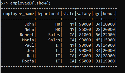
Let’s look into some more functionalities of Spark SQL. For that, we have to take a new DataFrame. Let’s create a new DataFrame with employee records.

employeeData =(('John','HR','NY',90000,34,10000),
('Neha','HR','NY',86000,28,20000),
('Robert','Sales','CA',81000,56,22000),
('Maria','Sales','CA',99000,45,15000),
('Paul','IT','NY',98000,38,14000),
('Jen','IT','CA',90000,34,20000),
('Raj','IT','CA',93000,28,28000),
('Pooja','IT','CA',95000,31,19000))
columns = ('employee_name','department','state','salary','age','bonus')
employeeDf = spark.createDataFrame(employeeData, columns)

If we wish to query the department wise total salary, we can achieve that in the following way:

employeeDf.groupby(col('department')).agg(sum(col('salary'))).show()

The result shows the department-wise total salary. If we want to see the total salary in an ordered way we can achieve by following way.

employeeDf.groupby(col('department')).agg(sum(col('salary')).alias('total_sal')).orderBy('total_sal').show()

Here, the total salary is appearing in ascending order. If we want to view this in descending order, we have to run the following command:

employeeDf.groupby(col('department')).agg(sum(col('salary')).alias('total_sal')).orderBy(col('total_sal').desc()).show()

We can perform group by and aggregate on multiple DataFrame columns at once:

employeeDf.groupby(col('department'),col('state')).agg(sum(col('bonus'))).show()

We can run more aggregates at one time by following way:

employeeDf.groupby(col('department')).agg(avg(col('salary')).alias('avarage_salary'),max(col('bonus')).alias('maximum_bonus')).show()

Windowing in Spark

Window functions allow us to calculate results such as the rank of a given row over a range of input rows

Suppose we want to calculate the second highest salary of each department. In such scenarios, we can use spark window functions.

To use windowing in spark, we have to import the Window package from pyspark.sql.window and then we can write the following

from pyspark.sql.window import Window
windowSpec = Window.partitionBy("department").orderBy(col("salary").desc())
employeeDf = employeeDf.withColumn("rank",dense_rank().over(windowSpec))
employeeDf.filter(col('rank') == 2).show()

In the above sequence of commands, first, we have imported the Window package from pyspark.sql.window.

Then we have defined the specification for windowing.

Next, we have performed the window function of DataFrame and added a new column rank that shows the highest salary per department.

Finally, we ran a command to show the second highest salary from all departments by filtering the DataFrame where the rank is 2.

Joins in Spark

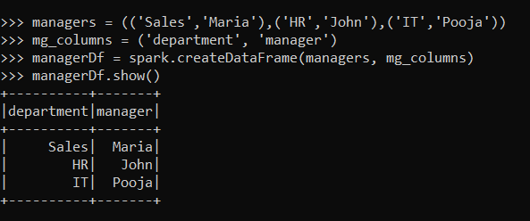
To perform join let’s create another dataset containing managers of each department.

managers = (('Sales','Maria'),('HR','John'),('IT','Pooja'))
mg_columns = ('department', 'manager')
managerDf = spark.createDataFrame(managers, mg_columns)
managerDf.show()

Now, if we want to view the name of managers of each employee, we can run the following command:

employeeDf.join(managerDf, employeeDf['department'] == managerDf['department'], how='inner').select(col('employee_name'),col('manager')).show()

We can perform the join of two DataFrames by the join method. We have to specify the columns on which we will be performing the join and the type of join we want to perform (inner, left, right, etc.) within the join method

Conclusion

In this article, we have learned the basics of Spark SQL, why it works lightning fast and how to manipulate spark DataFrames using Spark SQL. Also, we have learned to partition the data and order them logically and finally, how we can work with multiple DataFrames using join.

Thank you for reading. Hope these skills will help you to perform complex analysis on your data at speed.

Happy Learning!!