Building a simple Machine Learning model using Pytorch from scratch.

Introduction
Gradient descent is an optimization algorithm that is used to train machine learning models and is now used in a neural network. Training data helps the model learn over time as gradient descent act as an automatic system that tunes parameters to achieve better results. These parameters are updated after each iteration until the function achieves the smallest possible error. IBM
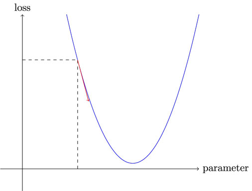
The red arrow in the figure below is a gradient and by updating our parameters after each iteration we can reduce loss which is our primary goal.

Gradient Descent
According to Arthur Samuel, gradient descent is the automatic processing of altering weights to maximize performance Fast AI. To be more specific, we will be discussing every step he processed that is required to turn function into a machine learning model.
- Initialize: We initialize the parameters to random values. These initial weights are the starting point of our model so that we can determine how far we are from our goal by using the loss function.
- Loss: We need a function that will take actual values and predicted values to calculate the error metric. The most common loss function is Mean Squared Error.
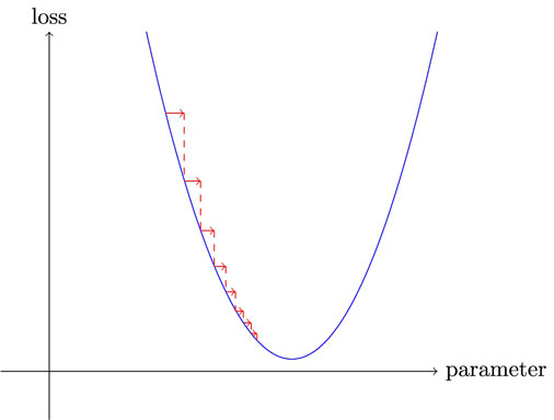
- Step: We are going to figure out what works best by increase or decreasing a small amount of weight to check if the loss went up or down. This method is not efficient as finding the correct direction takes time. This is where gradient comes to our rescue. The gradient slows us to figure out in which direction we should change weights to get better results. We have pass initial weights through functions to predict the values and using it calculate the loss. Then we take the gradient of our parameters and subtract it from our original parameters. This process repeats until you achieve the best possible score.
- Stop: We need to decide how many Epochs are required to train the model. These iterations will come to an end after that.

Code
The code is influenced by Jeremy Howard’s deep learning course Paperspace + Fast.AI . We will be using Pytorch for Model and Pyplot for visualization. Finally setting manual seed to reproduce the results. If you are using the Deepnote environment, you can copy and paste my code to get equivalent results.
import torch
import matplotlib.pyplot as plt
torch.manual_seed(2021);
Generating Values
X an integer series from 0 to 19. We can generate by using torch.arrange(start,end)
time = torch.arange(0,20).float()
time
tensor([ 0.,  1.,  2.,  3.,  4.,  5.,  6.,  7.,  8.,  9., 10., 11., 12., 13.,
        14., 15., 16., 17., 18., 19.])
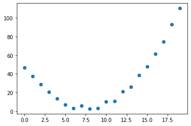
Y is calculated by using the quadratic function. We have added random noise in the code to make it look like real data.

speed = torch.rand(20)*5 +0.8*(time-7.5)**2+1
plt.scatter(time,speed);

Core Functions
Find a function that matches our observations. We are using generic quadratic functions as it’s hard to consider all possible functions.

our function takes two parameters, the t & params. Gradient Descent will be changing these parameters to improve the performance of our model.
def function(t,params):
  a,b,c = params
  return a*(t**2)+(b*t)+c
We will be using mean squared error (MSE) for loss function and root mean squared error (RMSE) for performance metrics. MSE is calculated by taking the average squared of difference between the predicted value and actual value.

def mse(preds,targets):
    return ((preds-targets)**2).mean()
Learning Rate
The learning rate is a step size for updating parameters at each iteration while moving toward minimizing loss. If the learning rate is too low it will take many steps to get the best result and on the other hand, if you select too high, it may bounce around rather than diverging. The best practice is to start small and then change it after each run to achieve minimum loss.

Setting initial weights by using torch.randn(3) and tell PyTorch that we want to track their gradients by using requires_grad_. Secondly, we are setting the learning rate to 1e-5. Lastly, we need to create a clone of the original parameters so that we can use it later to showcase accuracy metrics.
torch.randn(3).requires_grad_()
tensor([-2.3055, 0.9176, 1.5674], requires_grad=True)
params = torch.randn(3).requires_grad_()
orig_params = params.clone()
lr = 1e-5
Visualization
The visualization function compares the scatter plot of predicted and actual values.
def show_preds_actual(preds, ax=None):
    if ax is None: ax=plt.subplots()[1]
    ax.scatter(time, speed)
    ax.scatter(time, preds.detach().numpy(), color='red')
    ax.set_ylim(-100,100)
Let’s add initial parameters to our function and try to predict output and plot using matplotlib.pyplot. As we can see both are going in opposite directions. Next, we are going to use gradient descent to reduce the difference between the two functions.
preds = function(time, params)
show_preds_actual(preds)
.png)
Machine Learning Model
We are going to use the Arthur Samuel machine learning model that changes parameters to reduce loss automatically.
- Initialize weights using function
- Calculate loss
- Using parameters.required_grads_ allows us to call backwards on loss and then help us calculate the gradient of parameters.
- Calculate the gradient of parameters by multiplying it with the learning rate and then subtract it with the original parameters.
- Reset the gradients of the parameters
- Print RMSE
- Return prediction
def apply_step(params,prn=True):
  preds= function(time, params)
  loss = mse(preds, speed)
  loss.backward()
  params.data -= lr*params.grad.data
  params.grad = None
  if prn : print("RMSE:",(loss.item())**0.5)
  return preds
let’s run it for 6 iterations and see the results as the comparison between actual and predicted. As we can see with every iteration the red scatter plot which is the predicted function is slowly mimicking our actual function.
_,axs = plt.subplots(1,6,figsize=(12,3))
for ax in axs: show_preds_actual(apply_step(params, False), ax)
plt.tight_layout()
.png)
Now we need to reset our parameters using orig_params. We will run 10 iterations and print out RMSE. As we can see after the 4th iteration the RMSE metric is stable and reducing slowly.
params = orig_params.detach().requires_grad_()
for i in range(10) : preds = apply_step(params)
RMSE: 74.96194346966999
RMSE: 36.43029986215973
RMSE: 22.692756149058336
RMSE: 19.006926227796704
RMSE: 18.225665028268686
RMSE: 18.073917779669408
RMSE: 18.04494798288646
RMSE: 18.039351786874853
RMSE: 18.03818276871748
RMSE: 18.037850320630035
Conclusion
I used to think that you can build the machine learning model without going deep into the mechanism and it turns out my strategy had flaws as I was limited to existing models and libraries. If you want to create your own cutting-edge deep learning model you need to learn the mechanism of how neural networks works. You don’t need to learn mathematics but learning the smallest building blocks will help you create your model that will even perform better than the existing model.
In this tutorial, we have learned how Gradient decent works in deep learning, and by using Arthur Samuel’s original framework we have produced our model and train our data on that model. We have also evaluated our results by comparing visualization and RMSE metric score.
Learning Resources
- Practical Deep Learning for Coders | Practical Deep Learning for Coders (fast.ai)
- Deep Learning for Coders with Fastai and PyTorch: AI Applications Without a PhD: Howard, Jeremy, Gugger, Sylvain
- PyTorch for Deep Learning — Full Course / Tutorial — YouTube
I am Technology Manager turned Data Scientist, who loves building machine learning models and research on latest AI technologies. I am currently testing AI Products at PEC-PITC, which later get approved for human trials, eg: Breast Cancer Classifier.
You can follow me on LinkedIn and Polywork where I post amazing articles on Data Science and Machine Learning.


