This article was published as a part of the Data Science Blogathon
Introduction
The purpose of this article is to understand what is granger causality and its application in Time series forecasting for better prediction.
Image Source: https://www.wallpaperflare.com
Overview of Time series:
Time series is a set of observations on the values that the variable takes at different times. The time interval at which the data is collected may be hourly, daily, weekly, monthly, quarterly, annually, etc.
Time series data can be categorized as follows:
- Univariate time series – Consists of a single variable that changes over time. Eg Account balance over a span of ten years.
- Multivariate time series – Consists of more than one variable which varies over time and there may be dependency among the variables. Eg Different expenditures of a family over a span of ten years.
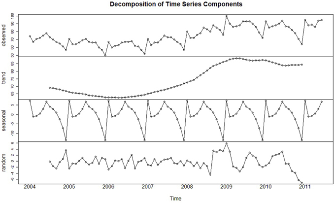
Time series analysis provides insight into the pattern or characteristics of time series data. Time series data can be decomposed into three components:
- Trend – This shows the tendency of the data over a long period of time, it may be upward, downward, or stable.
- Seasonality – It is the variation that occurs in a periodic manner and repeats each year.
- Noise or Random – Fluctuations in the data that are erratic.

Image Source: https://www.researchgate.net
Forecasting the data for a particular time in the future is known as Time Series Forecasting. It is one of the powerful machine learning models widely used in the fields like finance, weather forecasting, the health sector, environmental studies, business, retail, etc to arrive at strategic decisions.
In real-time, most of the data consists of multiple variables, in which independent variables might depend on other independent variables, these relations will have an impact on the predictions or forecasting. Most of the time people generally get misled and build multilinear regression models in such cases. A High R square value will further mislead and make a poor prediction.
Spurious Regression
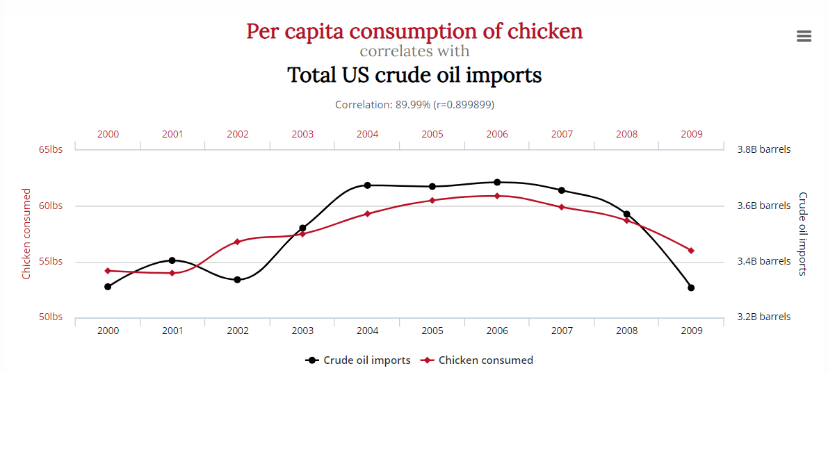
Linear regression might indicate a strong relationship between two or more variables, but these variables may be totally unrelated in reality. Predictions fail when it comes to domain knowledge, this scenario is known as spurious regression.
There is a strong relationship between chicken consumption and crude oil exports in the below graph even though they are unrelated.

Source: http://www.tylervigen.com/spurious-correlations
Strong trend / nonstationary and higher R square are observed in spurious regression. Spurious regression has to be eliminated while building the model since they are unrelated and have no causal relationship.
Multilinear regression makes use of a correlation matrix to check the dependency between all the independent variables. If the correlation coefficient value is high between two variables any one variable is retained and another one is discarded to remove the dependency. In the dataset when time is a confounding factor multilinear regression fails, the correlation coefficient which is used to eliminate the variable is not time-bound instead it just gives the correlation between the two variables.

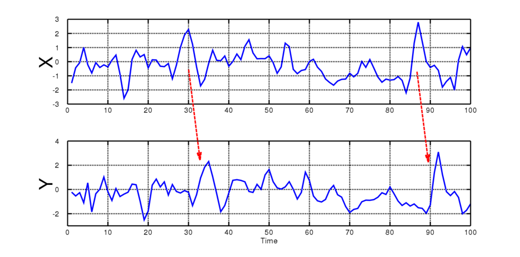
Consider the above time-series graph, variable X has a direct influence on variable Y but there is a lag of 5 between X and Y in which case we cant use the correlation matrix. For eg. an increase in coronavirus positive cases in the city and an increase in the number of people getting hospitalized. For better forecasting, here we would like to know if there is a causal relationship.

Image Source: https://clockwise.software/blog/solve-the-chicken-and-egg-problem/
Granger Causality comes to Rescue
Prof. Clive W.J. Granger, recipient of the 2003 Nobel Prize in Economics developed the concept of causality to improve the performance of forecasting.
It is basically an econometric hypothetical test for verifying the usage of one variable in forecasting another in multivariate time series data with a particular lag.
Granger causality is a statistical concept used to determine whether one time series can predict the future values of another time series. It measures the extent to which the past values of one variable provide valuable information for forecasting the other variable’s future behavior. Granger causality helps analyze potential relationships between variables, aiding in predicting trends. However, it’s important to note that Granger causality doesn’t prove direct causation and should be interpreted cautiously when evaluating causal relationships between variables.
A prerequisite for performing the Granger Causality test is that the data need to be stationary i.e it should have a constant mean, constant variance, and no seasonal component. Transform the non-stationary data to stationary data by differencing it, either first-order or second-order differencing. Do not proceed with the Granger causality test if the data is not stationary after second-order differencing.
Let us consider three variables Xt , Yt , and Wt preset in time series data.
Case 1: Forecast Xt+1 based on past values Xt .
Case 2: Forecast Xt+1 based on past values Xt and Yt.
Case3 : Forecast Xt+1 based on past values Xt , Yt , and Wt, where variable Yt has direct dependency on variable Wt.
Here Case 1 is univariate time series also known as the autoregressive model in which there is a single variable and forecasting is done based on the same variable lagged by say order p.
The equation for the Auto-regressive model of order p (RESTRICTED MODEL, RM)
Xt = α + 𝛾1 X𝑡−1 + 𝛾2X𝑡−2 + ⋯ + 𝛾𝑝X𝑡−𝑝
where p parameters (degrees of freedom) to be estimated.
In Case 2 the past values of Y contain information for forecasting Xt+1. Yt is said to “Granger cause” Xt+1 provided Yt occurs before Xt+1 and it contains data for forecasting Xt+1.
Equation using a predictor Yt (UNRESTRICTED MODEL, UM)
Xt = α + 𝛾1 X𝑡−1 + 𝛾2X𝑡−2 + ⋯ + 𝛾𝑝X𝑡−𝑝 + α1Yt-1+ ⋯ + α𝑝 Yt-p
2p parameters (degrees of freedom) to be estimated.
If Yt causes Xt, then Y must precede X which implies:
- Lagged values of Y should be significantly related to X.
- Lagged values of X should not be significantly related to Y.
Case 3 can not be used to find Granger causality since variable Yt is influenced by variable Wt.
Hypothesis test
Null Hypothesis (H0) : Yt does not “Granger cause” Xt+1 i.e., 𝛼1 = 𝛼2 = ⋯ = 𝛼𝑝 = 0
Alternate Hypothesis(HA): Yt does “Granger cause” Xt+1, i.e., at least one of the lags of Y is significant.
Calculate the f-statistic
Fp,n-2𝑝−1 = (𝐸𝑠𝑡𝑖𝑚𝑎𝑡𝑒 𝑜𝑓 𝐸𝑥𝑝𝑙𝑎𝑖𝑛𝑒𝑑 𝑉𝑎𝑟𝑖𝑎𝑛𝑐𝑒) / (𝐸𝑠𝑡𝑖𝑚𝑎𝑡𝑒 𝑜𝑓 𝑈𝑛𝑒𝑥𝑝𝑙𝑎𝑖𝑛𝑒𝑑 𝑉𝑎𝑟𝑖𝑎𝑛𝑐𝑒)
Fp,n-2𝑝−1 = ( (𝑆𝑆𝐸𝑅𝑀−𝑆𝑆𝐸𝑈𝑀) /𝑝) /(𝑆𝑆𝐸𝑈𝑀 /𝑛−2𝑝−1)
where n is the number of observations and
SSE is Sum of Squared Errors.
If the p-values are less than a significance level (0.05) for at least one of the lags then reject the null hypothesis.
Perform test for both the direction Xt->Yt and Yt->Xt.
Try different lags (p). The optimal lag can be determined using AIC.
Limitation
- Granger causality does not provide any insight on the relationship between the variable hence it is not true causality unlike ’cause and effect’ analysis.
- Granger causality fails to forecast when there is an interdependency between two or more variables (as stated in Case 3).
- Granger causality test can’t be performed on non-stationary data.
Resolving Chicken and Egg problem
Let us apply Granger causality to check whether the egg came first or chicken came first.
Importing libraries
import matplotlib.pyplot as plt
 import seaborn as sns
 import numpy as np
 import pandas as pd
Loading Dataset
Data is from the U.S. Department of Agriculture. It consists of two-time series variables from 1930 to 1983, one of U.S. egg production and the other the estimated U.S. chicken population.
df = pd.read_csv('chickegg.csv')
Exploring the Dataset
df.head()
df.dtypes
df.shape
(53, 3)
df.describe()
Check if the data is stationary, if not make it stationary to proceed.
# Draw Plot
def plot_df(df, x, y, title="", xlabel='Date', ylabel='Value', dpi=100):
    plt.figure(figsize=(16,5), dpi=dpi)
    plt.plot(x, y, color='tab:red')
    plt.gca().set(title=title, xlabel=xlabel, ylabel=ylabel)
    plt.show()
plot_df(df, x=df.Year, y=df.chicken, title='Polulation of the chicken across US')
plot_df(df, x=df.Year, y=df.egg, title='Egg Produciton')
By visual inspection, both the chicken and egg data are not stationary. Let us confirm this by running Augmented Dickey-Fuller Test (ADF Test).
Augmented Dickey-Fuller Test (ADF test)
ADF test is a popular statistical test for checking whether the Time Series is stationary or not which works based on the unit root test. The number of unit roots present in the series indicates the number of differencing operations that are required to make it stationary
Consider the hypothesis test where:
Null Hypothesis (H0): Series has a unit root and is non-stationary.
Alternative Hypothesis (HA): Series has no unit root and is stationary.
from statsmodels.tsa.stattools import adfuller
result = adfuller(df['chicken'])
print(f'Test Statistics: {result[0]}')
print(f'p-value: {result[1]}')
print(f'critical_values: {result[4]}')
if result[1] > 0.05:
    print("Series is not stationary")
else:
    print("Series is stationary")
result = adfuller(df['egg'])
print(f'Test Statistics: {result[0]}')
print(f'p-value: {result[1]}')
print(f'critical_values: {result[4]}')
if result[1] > 0.05:
    print("Series is not stationary")
else:
    print("Series is stationary")
p-values of both the egg and chicken variables are greater than the significant value (0.05), the Null hypothesis is valid and the series is not stationary.
Data Transformation
Granger causality test is carried out only on stationary data hence we need to transform the data by differencing it to make it stationary. Let us perform the first-order differencing on chicken and egg data.
df_transformed = df.diff().dropna()
df = df.iloc[1:]
print(df.shape)
df_transformed.shape
df_transformed.head()
plot_df(df_transformed, x=df.Year, y=df_transformed.chicken, title='Polulation of the chicken across US')
plot_df(df_transformed, x=df.Year, y=df_transformed.egg, title='Egg Produciton')
Repeat the ADF test again on differenced data to check for stationarity.
result = adfuller(df_transformed['chicken'])
print(f'Test Statistics: {result[0]}')
print(f'p-value: {result[1]}')
print(f'critical_values: {result[4]}')
if result[1] > 0.05:
    print("Series is not stationary")
else:
    print("Series is stationary")
result = adfuller(df_transformed['egg'])
print(f'Test Statistics: {result[0]}')
print(f'p-value: {result[1]}')
print(f'critical_values: {result[4]}')
if result[1] > 0.05:
    print("Series is not stationary")
else:
    print("Series is stationary")
Transformed chicken and egg data are stationary, hence there is no need to go for second-order differencing.
Test the Granger Causality
There are several ways to find the optimal lag but for simplicity let’s consider 4th lag as of now.
Do eggs granger cause chickens?
Null Hypothesis (H0) : eggs do not granger cause chicken.
Alternative Hypothesis (HA) : eggs granger cause chicken.
from statsmodels.tsa.stattools import grangercausalitytests
grangercausalitytests(df_transformed[['chicken', 'egg']], maxlag=4)
p-value is very low, Null hypothesis is rejected hence eggs are granger causing chicken.
That implies eggs came first.
Now repeat the Granger causality test in the opposite direction.
Do chickens granger cause eggs at lag 4?
Null Hypothesis (H0) : chicken does not granger cause eggs.
Alternative Hypothesis (HA) : chicken granger causes eggs.
grangercausalitytests(df_transformed[['egg', 'chicken']], maxlag=4)
The p-value is considerably high thus chickens do not granger cause eggs.
The above analysis concludes that the egg came first and not the chicken.
Once the analysis is done the next step is to begin forecasting using time series forecasting models.
Frequently Asked Questions
A. Granger causality is a statistical concept used to determine if one time series can predict another’s future values. If a time series A Granger-causes another time series B, it means that past values of A provide useful information in predicting future values of B, beyond what B’s own past values provide. This concept is widely applied in econometrics, neuroscience, and more. However, Granger causality doesn’t imply true causation; it only suggests a predictive relationship. Both variables’ behavior and external factors should be considered to draw meaningful conclusions about causal relationships.
A. Granger causality between two variables suggests that the past values of one variable provide predictive information about the future values of another variable, beyond the information contained in its own past values. It’s a statistical approach to assess temporal relationships but doesn’t imply direct causation; rather, it indicates whether one variable helps predict the other.
EndNote
Whenever you come across time-bound data having multiple variables be suspicious about high R2 and possible spurious regression. Make use of the time series forecasting for better performance. Check for bidirectional Granger causality between each variable and eliminate the variable based on test results before proceeding with forecasting techniques. I hope you enjoyed the article and gained insight into the Granger causality concept. Please drop your suggestions or queries in the comment section.
Thank you for reading!
About Author
Hello, Pallavi Padav from Mangalore holding PG degree in Data Science from INSOFE. Passionate about participating in Data Science hackathons, blogathons and workshops.
The media shown in this article are not owned by Analytics Vidhya and are used at the Author’s discretion.
.jpg)


Very well written and explained.
I have really enjoyed this article, so simply writen and yet so precise. Congratulations
chickegg.csv, could you please share the data???