This article was published as a part of the Data Science Blogathon
Overview
- Deep learning is a subset of Machine Learning dealing with different neural networks with three or more layers.
- There are different deep neural networks that work best on many different real-world applications and research and development are still going on.
- The comprehensive guide will introduce different methods we should take care of and use while working and building neural network models to get better results.
Introduction
Machine Learning algorithms are not able to train on huge datasets, Image datasets, textual data. Neural networks being the heart of deep learning provides a state of accuracy in many of these use cases. What truly fascinates about a neural network is there working and capability to learn complex things.
But most of the time the network model we build might not give satisfactory results or might not take us to top positions on the leaderboard in data science competitions. As a result, we always look for a way to improve the performance of neural networks.

In this article, we are going to understand the problem neural networks faced in different situations and a solution that works best to get better results. I would like to request you to try and implement all the methods once we will study.
Table of Contents
- Vanishing Gradient Descent Problem
- Defining Neural Network Architecture
- Why does Weight Initialization matter?
- Control Neural Network Overfitting
- Reduce Complexity
- Dropout Layers
- Early Stopping
- Normalization
- Monitor Your Gradients(Gradient Clipping)
- Hyperparameter Tuning of Neural Network
Vanishing Gradient Problem for Neural Networks Performance Optimization
Gradient Descent is an iterative optimization algorithm for finding the local minimum of an input function. It is also known as the steepest descent. Why is it known as gradient? A gradient is nothing but a derivative. it’s a derivative of loss with respect to weights. Gradient descent performs two steps iteratively. The first is to compute the gradient mean slope and the second is to move a step opposite in direction of the slope.
Neural networks are not a new technology; they were being used in the 1980s also, but in that period developing a deep neural network was not possible because the activation function we used is the sigmoid function. What is a problem with the Sigmoid function is that it gives a problem of vanishing gradient descent. The sigmoid function is a function that normalizes any value in the range of 0 to 1. And when you find its derivative, its range is always between 0 to 0.25, which can be observed by the below graph. we find its derivative so that we can apply gradient descent to update weights and formula is.
W_new = W_old – learning_rate * derivate of loss with weight
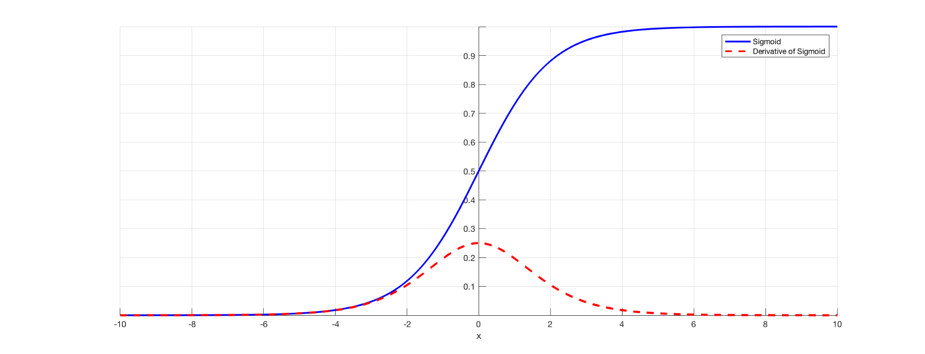
Hence the value of a derivative is decreasing so when we update the weights it happened very slowly because the derivative is too small and as we increase layers it continuously decreasing and after 2 layers of neural network updating weights does not make any sense because the new weight is equal to the old weight. And this situation is known as Vanishing Gradient Problem. In simple words vanishing gradient refers to the fact that in backpropagation gradients typically decrease exponentially as a function of distance from the last layer. Hence, before 1986, people were not able to implement deep neural networks. To solve this problem, we use the recently published activation function as Relu.
How Relu solves the problem of Vanishing Gradient Descent?
ReLU stands for a Rectified linear unit that has a gradient of 1 when input is greater than zero; otherwise, it is zero. In a short period of time, ReLU has become the default and most favorite activation function of most people that make training a neural network easier and helps to achieve better performance.
g(z) = max(0, z)
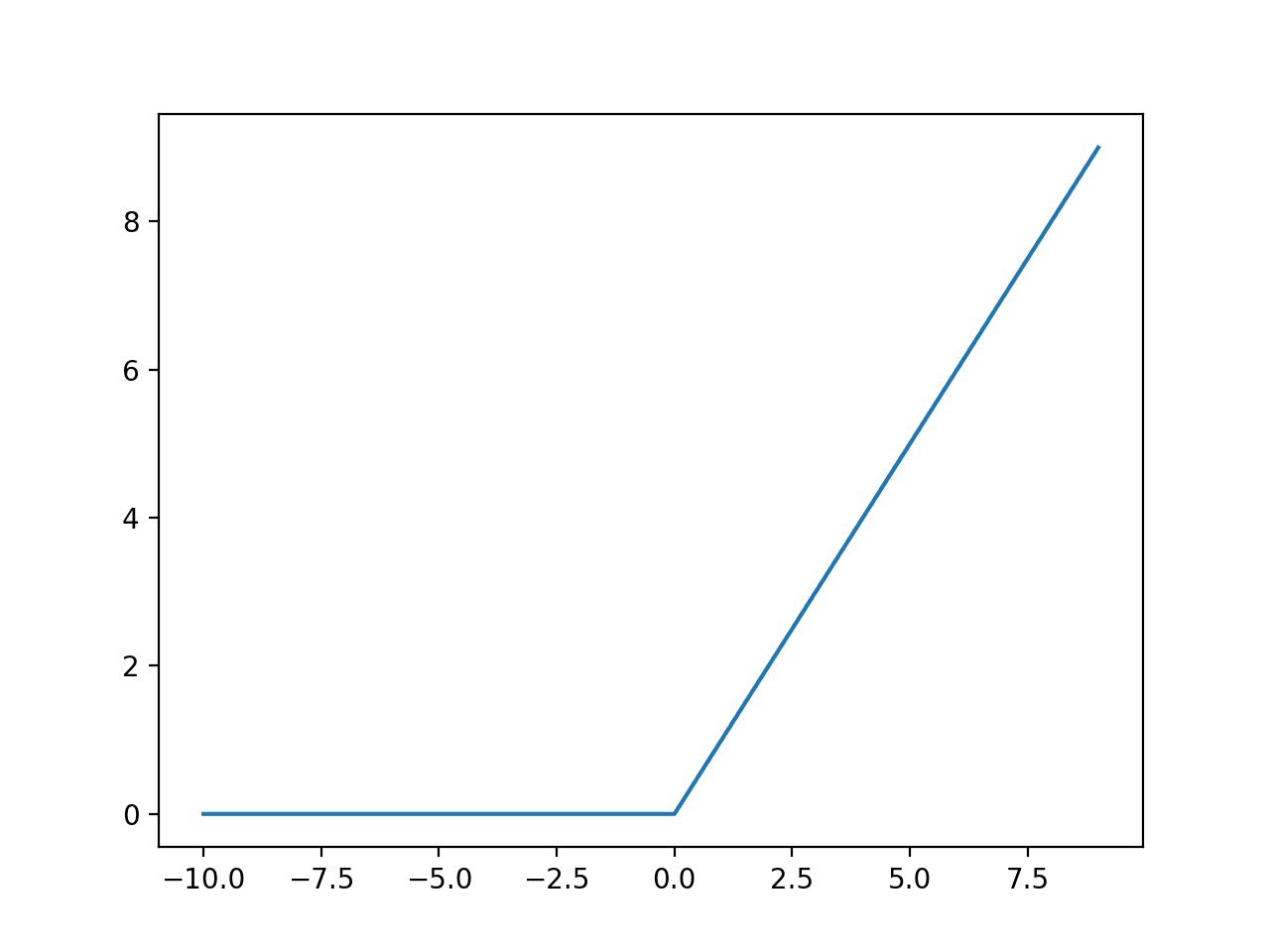
What can we derive from ReLu? The ReLU function does not saturate, and it has a bigger and constant gradient as compared to the sigmoid and tanh activation functions. The function is linear for values greater than zero, and it is non-linear for negative values.
when we multiply a bunch of relative derivatives together in backpropagation, then it has the nice property of being either 1 or 0. Hence, there is no vanishing or diminishing gradient descent.
Defining Neural Network Architecture for Neural Networks Performance Optimization
There are some common things that we know while building a neural network, but it’s necessary to remember such parameters working with a different problem statement
I) Loss Function
- With the Binary Classification problem statement, we use binary cross-entropy as a loss function
- In the multi-class classification problem, we use sparse categorical cross-entropy
- In Regression, we use mean squared error
ii) Optimizers to choose
The best performance optimizer currently used in many use cases is Adam. Apart from it, there are many great optimizers like RMSProp, Adagrad, Adadelta, etc.
iii) Activation Function
- In neural network architectures with hidden layers, relu is the most preferred activation function.
- In last layer working with binary classification use sigmoid
- In last layer working with Multiclass classification use softmax
- In Regression problems use linear
There is some other activation function like tanh that also sometimes works effectively.
Proper Weight Initialization for Neural Networks Performance Optimization
Weight initialization comprises setting up the weights vector for all the neurons for the first time just before neural network training starts. A network with improper weight initialization makes the learning process complex, and time-consuming; therefore, to achieve faster convergence and feasible learning weight initialization matters. There are different ways people use for weight initialization and let’s see which method creates a problem and which to use in different scenarios.
i) Initializing weights with zero
It is possible to initialize weights with zero, but it is a bad idea to do so because initializing weights with zero creates no sense of building a neural network if the neurons are dead on the initial state. It makes the model work equivalent to a linear model.
ii) Random Initialization
To randomly initialize the weights, you can use 2 statistical methods as the standard normal distribution or uniform distribution. In random initialization, weights are greater than 0, and neurons aren’t dead. with the random initialization, you will observe exponentially decreasing loss but then inverted and we can encounter the problem of vanishing gradient descent or exploding gradient descent.
we have seen that initializing weights with zero or random initializing is not good. let’s discuss some standard methods that prove to be best for weight initialization.
iii) Xavier Initialization
Deep learning models find it difficult to converge when weights are initialized with normal distribution. This is because the variance of weights is not taken care of, which leads to large or very small activation values and result in exploding gradient problems. In order to overcome this problem, Xavier initialization was introduced that keeps the variance of all layers equal.
This is an inbuilt method in Keras to initialize weights implemented by a computer scientist name Gloret Xavier. It uses some specific statistical methods to define weights for neurons. The Xavier initialization method is calculated as a random number with a uniform probability distribution (U) between the range -(1/sqrt(n)) and 1/sqrt(n), where n is the number of inputs to a node. In Xavier initialization biases are initialized with zero and weights are initialized as.
weight = U [-(1/sqrt(n)), 1/sqrt(n)]
As a rule of thumb, Xavier initialization works best with the sigmoid or tanh activation function. If you want to derive the complete formula and understand Xavier’s initialization in detail please refer to andy’s blog here.
iv) He Initialization.
Kaiming Initialization or He Initialization is the weight initialization method for neural networks that takes into account the non-linearity of activation functions, such as ReLU activation.
If you are working with relu activation then He initializer with giving better results that brings the variance of outputs to approximately one. It is the same as Xavier, the difference is related to the non-linearities of Relu, which is non-differentiable at x=0. So with relu, it is better to initialize the weights with He initialization which defines variance using the below formula.
v^2 = 2/N
That is, a zero-centered Gaussian with a standard deviation of the square root of 2/N (variance shown in the equation above). Biases are initialized at 0. This is HE initialization. For more on Kaiming(He) Initialization please refer to this blog.
Control Overfitting of Neural Network for Performance Optimization
Overfitting happens when the model tends to learn noise or mesmerize the training data and performs well on training data but gives the worst performance on test data(new data) and this is called overfitting. Neural networks also undergo overfitting when you try to implement a deep network on small data or without using any type of regularization and applying a huge number of epochs. There are different methods to control overfitting in neural networks.
i) Reduce complexity/increase data
The easy way to reduce overfitting is by increasing the input data so that neural network training is on more high-dimensional data. A much as you increase the data, it will stop learning noise. If not possible to increase data, then try reducing the complexity of neural network architecture by reducing the number of hidden layers, reducing the number of nodes, decrease some number of epochs.
ii) Dropout Layers
Dropout is an interesting and new phenomenon to reduce overfitting in neural networks. I hope that you know the decision tree. The problem with the decision tree is that it overfits the data, and the solution to this came with a random forest. In a random forest algorithm, we built different decision trees and each decision tree gets the sample data instead of complete data, which prevents the model from overfitting in such a way that all the noise has not been learned by each model. In simple words, we perform regularization by randomization in a random forest and prevent overfitting.
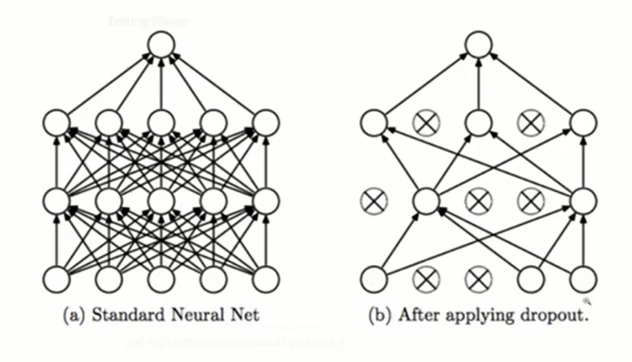
The same method is used by dropouts in neural networks. In each epoch, dropout inactivates a certain number of the neurons needed to take part in the training. The neurons are selected on a random basis. We declare a rate with dropout while using describe the probability of neurons not being selected in the training set. 0.2 to 0.5 rate values are mostly used and provide better results.
iii) Regularization(L1 and L2)
L1 and L2 regularization are also powerful machine learning regularization techniques you can use to punish neural network training and reduce overfitting.
Majorly, in the neural network, we use lasso(L1) regularization. In L1 and L2 regularization we add a regularization parameter that tries to minimize weights. And due to this correction in weights, some connections in the network are breaking, and first, where the model was trying to catch all the connections, now due to adding regularization parameter, it will try to smoothen the loss.
The equation SGD is
new_weight = old_weight – LR * gradient
After applying L1 regularization the equation becomes
new_weight = old_weight(1 – LR * alpha) – LR * gradient
If you look at both equations then they are the same, only one extra term is introduced. If the value of alpha is high, then the value of weights will reduce. And overfitting happens only when weights attain a high value, and by using this we are capable of handling the value of weights and reducing overfitting.
While implementing this in the neural network there is a parameter called kernel initializer. we use this to define the type of regularization to use.
model = Sequential()
model.add(Dense(128, input_dim=2, activation="relu", kernel_regularizer='l2'))
model.add(Dense(1, input_dim=2, activation="sigmoid", kernel_regularizer='l2'))
model.compile(loss='binary_crossentropy',optimizer='adam',metrics=['accuracy'])
iv) Early Stopping
Early stopping is a method where we apply a constraint on training neural networks. It strictly prevents the training of deep neural networks by stopping the training at a certain moment and terminating the code. Have a look at the below graph to understand early stopping. When a model overfits data, then the loss graph you obtained is something like the below graph.
We can observe that training error is decreasing, but what about test error, it is decreasing first and after 750 to 800 epochs it gradually starts increasing, which means the neural network is overfitting the data. Here, early stopping criteria help us to improve the model. What early stopping does is from the point where test error starts increasing, it will stop the training before the point where the error was minimum and the graph will not move forward.
To implement early stopping practically white, we train neural networks, there is a method called callback that can be used and we can pass the Early stopping function to it which will monitor the validation loss continuously and will stop training where it seems to be increasing.
history = model.fit(x_train, y_train, validation_data = (x_test, y_test),epochs = 200,
callbacks = EarlyStopping(monitor="val_loss"))
After using early stopping you will get a smooth boundary and control overfitting. As I have plotted then observe below graph, it stops after 100 epochs mean where test loss is minimum, it will stop there, that is early stopping.

- For more on Early Stopping Please refer to Wikipedia Article
- More on overfitting in Neural Networks, Refer to this blog.
Why is Normalization important in Neural networks?
Normalization is a technique used in the data preprocessing step to bring the value of the numeric column in a common scale-like between 0 to 1 or -1 to 1. Normalizing the values makes it easy for most machine learning algorithms to run faster and achieve better performance.
It’s been said that whenever you pass the data to a neural network first, you should Normalize them. When data is not normalized it is not the case that the neural network will not converge, but it will slow down the process and need a huge number of epochs to converge. In simple words, the accuracy and convergence you can get with normalized data in 200 epochs cannot achieve them even in 2000 epochs. Let’s prove this Practically why the normalization of values matters working with neural networks.
We will be using the Pima Indians Diabetes dataset available on Kaggle. The dataset is simple and popular where we have to predict whether a person has diabetes or not using some features like insulin level, BMI, age, many different features. the dataset looks like the below sample image.
We will compare the performance of the neural network when without normalization data is passed and with normalization, data is passed. Below is the architecture of the neural network where data after splitting in train and test passes to model without normalizing.
model = Sequential()
model.add(Dense(10,input_dim=2, activation="relu"))
model.add(Dense(10, activation="relu"))
model.add(Dense(1, activation="sigmoid"))
model.compile(loss="binary_crossentropy", optimizer="adam", metrics=['accuracy'])
history = model.fit(x_train, y_train, validation_data=(x_test, y_test), verbose=1)
import matplotlib.pyplot as plt
plt.plot(history.history['val_accuracy'])
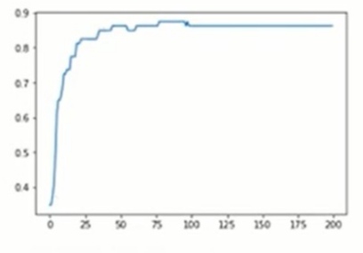
You can see in the above graph that the model is not able to converge even after the end of epochs and it is varying between 72 and 27. When we pass the data after normalization then our results are better as compared to the above case.
from sklearn.preprocessing import StandardScaler
scaler = StandardScaler()
X = scaler.fit_transform(X)
from sklearn.model_selection import train_test_split
X_train,X_test,y_train,y_test = train_test_split(X,y,test_size=0.2,random_state=1)
Now pass data to the same model created above and observe the results.
Monitor your gradients(Gradient clipping)
Gradient Clipping means forcing a value of gradient to a specific minimum or maximum when the gradient exceeded an expected range. It is known as Gradient Clipping. This is a way of preventing a gradient from exploding and going out of control in deep architecture- especially in RNNs and CNNs. In simple words whenever the Gradient descent algorithm tries to take a long step, the gradient clipping prevents it to reduce the step size so that it is less likely to go outside the region. Keras optimizer has two parameters or there are two approaches to do so.
i) Clip by norm ~ If the L2 norm or gradient tensor is more than a specific value, we normalize the gradient tensor with the below equation. It is we divide the old gradient with its modulus into clip norm parameters.
gradient = gradient * clipnorm / ||gradient||
ii) Clip by value ~ If the value at any index in gradient tensor is greater than a specific value or less than zero or the same negative value, we normalize the gradient using the below equation.
gradient = clip(gradient, -clipvalue, clipvalue)
It is recommended to use clipping by norm as the direction of the gradient won’t change after scaling. It means that when we use clip-by value then the direction of the steepest gradient has high chances of changing; that is not the case with clip-by-norm; thus the optimization remains stable.
we can simply implement this using Keras while initializing the I optimizer during model compilation.
model.compile(optimizer=Adam(learning_rate=0.1, clipnorm=1))
You can try clip by value too and compare the results. To read more on gradient clipping please visit this blog.
Hyperparameter Tuning of Deep Neural Network
There is a library called Keras-Tuner that you can use to select the right set of parameters to tune a neural network and improve its performance. We will practically learn hyperparameter tuning with Keras-tuner on some datasets. we are using the same Pima Indian Diabetes Dataset of Kaggle that we used above. We will perform hyperparameter tuning to select the right optimizer, number of nodes in a layer, number of layers.
How to Select the right optimizer using Keras-tuner?
Step-1) First, you need to install the Keras-tuner using the pip command.
pip install -U keras-tuner
Step-2) After installing, lets the loaded dataset and split the dataset into train and test set for building model.
import pandas as pd
df = pd.read_csv('diabetes.csv')
from sklearn.preprocessing import StandardScaler
from sklearn.model_selection import train_test_split
X = df.iloc[:,:-1].values
y = df.iloc[:,-1].values
scaler = StandardScaler()
X = scaler.fit_transform(X)
X_train,X_test,y_train,y_test = train_test_split(X,y,test_size=0.2,random_state=1)
Step-3) Building Model architecture for Hyperparameter Tuning
Now we will build a function that will build a model architecture with various sets of parameters we want to train the model upon and select the best set of parameters from it.
import tensorflow
from tensorflow import keras
from keras import Sequential
from keras.layers import Dense,Dropout
import kerastuner as kt
def build_model(hp):
  model = Sequential()
  model.add(Dense(32,activation='relu',input_dim=8))
  model.add(Dense(1,activation='sigmoid'))
  optimizer = hp.Choice('optimizer', values = ['adam','sgd','rmsprop','adadelta'])
  model.compile(optimizer=optimizer, loss='binary_crossentropy',metrics=['accuracy'])
  return model
We are tuning the model on top of the optimizer. After calling a build model function, it will return a compiled model object.
Step-4) Create Tuner Object
Now we will create a tuner object where we need to pass a model function, objective, and max trials. The objective here is to improve validation accuracy, and max trails mean how many times we want to iterate over parameters to choose the right parameter.
tuner = kt.RandomSearch(build_model,
                        objective='val_accuracy',
                        max_trials=5)
Now as you call a search function, it will start running epochs and display the results of each fit by using a different optimizer each time. To see the best hyperparameter use get the best hyperparameter function and access to zero index values.
tuner.search(X_train,y_train,epochs=5,validation_data=(X_test,y_test))
tuner.get_best_hyperparameters()[0].values
You will get the output in various trials as shown below, and by using the function get the best hyperparameter you can see the best parameter fit for the model.
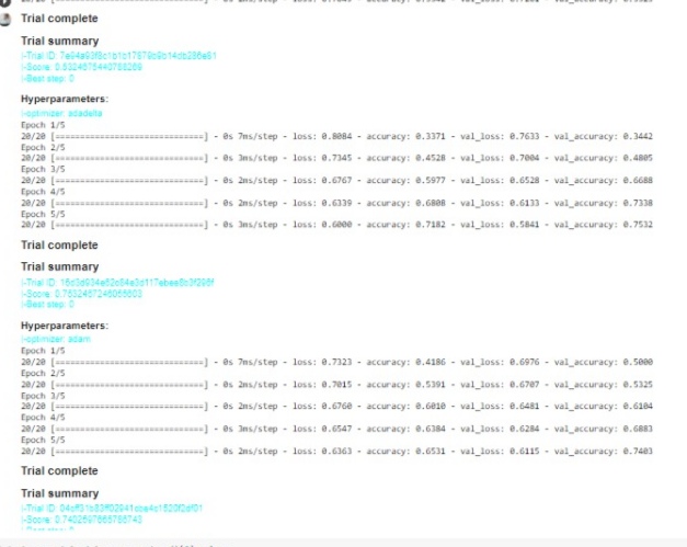
And if you directly want to retrieve the best model which is trained on the best hyperparameter so we can also do so, and use it directly for prediction.
model = tuner.get_best_models(num_models=1)[0]
model.summary()
It gives RMSProp, the best optimizer to use that gives 82 percent accuracy on a validation set. That’s how we use basic three to four steps to choose the right set of parameters. let’s do more.
How to find the number of nodes in a layer?
All steps are the same as we have studied above, so we will directly implement build a model function where we will use hyperparameter integer function to define a range. And we will create a tuner object and call the search function that starts iteration and displays the result by training a model on any random value in the range.
def build_model(hp):
  model = Sequential()
  units = hp.Int('units',min_value = 8,max_value = 128)
  model.add(Dense(units=units, activation='relu',input_dim=8))
  model.add(Dense(1,activation='sigmoid'))
  model.compile(optimizer='rmsprop',loss='binary_crossentropy',metrics=['accuracy'])
  return model
tuner = kt.RandomSearch(build_model,
                        objective='val_accuracy',
                        max_trials=5,
                        directory='mydir',
                        project_name='num_neurons')
tuner.search(X_train,y_train,epochs=5,validation_data=(X_test,y_test))
It gives 72 as the right number of neurons to be used in a layer. Now you can use get the best hyperparameter function to check the best fit.
How to select a number of layers?
There is a little bit of difference in creating a function for selecting layers than the above two functions because for selecting layers we need to run a loop so that when it will keep increasing layer one, be one in network architecture, train it and display results.
def build_model(hp):
  model = Sequential()
  model.add(Dense(72,activation='relu',input_dim=8))
  for i in range(hp.Int('num_layers',min_value=1,max_value=10)):
    model.add(Dense(72,activation='relu'))
  model.add(Dense(1,activation='sigmoid'))
  model.compile(optimizer='rmsprop',loss='binary_crossentropy',metrics=['accuracy'])
  return model
tuner = kt.RandomSearch(build_model,
                        objective='val_accuracy',
                        max_trials=3,
                        directory='mydir',
                        project_name='num_layers')
We get 6 as the best number of hidden layers in neural network architectures.
Combining all together
Now finally you will be thinking of hyperparameter tuning; we need to do this separately, so must say that’s not the case. Now we will be doing hyperparameter tuning in a single function to select the number of neurons in a layer, a number of layers, activation function, optimizer, and even the rate of dropout we should use.
def build_model(hp):
  model = Sequential()
  counter = 0
  for i in range(hp.Int('num_layers',min_value=1,max_value=10)):
    if counter == 0:
      model.add(Dense(hp.Int('units' + str(i), min_value=8, max_value=128,step=8),activation= hp.Choice('activation' + str(i), values=['relu','tanh','sigmoid']),input_dim=8))
      model.add(Dropout(hp.Choice('dropout' + str(i), values=[0.1,0.2,0.3,0.4,0.5,0.6])))
    else:
      model.add(Dense(hp.Int('units' + str(i), min_value=8, max_value=128,step=8),activation= hp.Choice('activation' + str(i), values=['relu','tanh','sigmoid'])))
      model.add(Dropout(hp.Choice('dropout' + str(i), values=[0.1,0.2,0.3,0.4,0.5,0.6])))
    counter+=1
  model.add(Dense(1,activation='sigmoid'))
  model.compile(optimizer=hp.Choice('optimizer',values=['rmsprop','adam','sgd','nadam','adadelta']),
                  loss='binary_crossentropy',
                  metrics=['accuracy'])
  return model
It gives pretty decent results, and the hyperparameter it generates for the model does not overfit anymore and the results are great. And now if you plot the accuracy and loss graph of the model you will get a smooth plot.
plt.figure(0)
plt.plot(history.history['accuracy'], label="Training accuracy")
plt.plot(history.history['val_accuracy'], label="val accuracy")
plt.title("Accuracy")
plt.xlabel("epochs")
plt.ylabel("accuracy")
plt.legend()
plt.figure(1)
plt.plot(history.history['loss'], label="training loss")
plt.plot(history.history['val_loss'], label="val loss")
plt.title("Loss")
plt.xlabel("epochs")
plt.ylabel("Loss")
plt.legend()
plt.show()
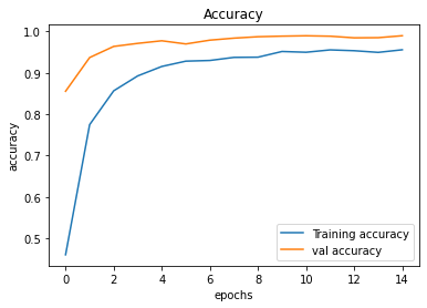
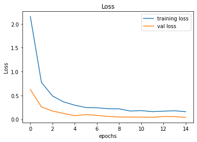
Keras-tuner is a great library you should play around it and use for choosing the right set of hyperparameters for your neural network model to control overfitting.
End Notes
In this article, we discussed different approaches and methods to improve the performance of neural networks. We looked at the challenges neural networks faced in different scenarios and the solution we should use to overcome them. we learned techniques like regularization, early stopping that can help to converge faster. Finally, we came across hyperparameter tuning, which is a crucial method to improve overall network architecture and performance, and we have performed hyperparameter tuning from scratch in different ways.
- For more on Improving the performance of Neural networks please refer official paper of Robert, Harris, and Patrice here.
- Practicals with improving deep learning model performance, Link
If you have any doubts or feedback, feel free to share them in the comments section below.
About The Author
I am pursuing a bachelor’s in computer science. I am a data science enthusiast and love to learn, work in data technologies.
Connect with me on Linkedin
Check out my other articles here and on Blogspot
Thanks for giving your time!
The media shown in this article are not owned by Analytics Vidhya and are used at the Author’s discretion.


In your build_model function, what is 'hp'?