Latent Semantic Analysis and its Uses in Natural Language Processing

Textual data, even though very important, vary considerably in lexical and morphological standpoints. Different people express themselves quite differently when it comes to texts and their choice of words may vary significantly without getting deviated from the theme. For example:

Latent Semantic Analysis (LSA) involves creating structured data from a collection of unstructured texts. Before getting into the concept of LSA, let us have a quick intuitive understanding of the concept. When we write anything like text, the words are not chosen randomly from a vocabulary.

Rather, we think about a theme (or topic) and then chose words such that we can express our thoughts to others in a more meaningful way. This theme or topic is usually considered as a latent dimension.

It is latent because we can’t see the dimension explicitly. Rather, we understand it only after going through the text. This means that most of the words are semantically linked to other words to express a theme. So, if words are occurring in a collection of documents with varying frequencies, it should indicate how different people try to express themselves using different words and different topics or themes.

In other words, word frequencies in different documents play a key role in extracting the latent topics. LSA tries to extract the dimensions using a machine learning algorithm called Singular Value Decomposition or SVD.

!wget http://mlg.ucd.ie/files/datasets/bbc-fulltext.zip
!unzip bbc-fulltext.zip
import pandas as pd
import os, re

# Read each file as text files and put in a data frame
folders = os.listdir('/content/bbc/')
folders

# OUTPUT: ['business', 'entertainment', 'README.TXT', 'sport', 'tech', 'politics']

folders = os.listdir('/content/bbc/')

folders.remove('README.TXT')

df_dict = {'topic':[], 'news':[]}

for folder in folders:

    files = os.listdir('/content/bbc/'+folder)

    for file in files:

        path = '/content/bbc/'+folder+'/'+file

        f = open(path, 'r', errors='ignore').read()

        df_dict['topic'].append(folder)

        df_dict['news'].append(str(f))




df = pd.DataFrame(df_dict)

df.head()

The news column contains the texts which require some preprocessing before further analysis. Preprocessing would involve steps like

• Case conversion
• Removal of special characters and numbers (if any)

Using the RE package this processing can be done easily. A convenient function can do preprocessing and, as the data contain news heading, the function will return both the heading as well as the actual news content from individual texts. The codes are given below:

def simple_preprocessing(text):
    heading = re.findall("^.+(?=\n)", text) # Extract the first line as heading
    text = re.sub(heading[0], '', text) # Remove the heading
    text = re.sub('\n', ' ', text) # Replace newline character with whitespace
    text = re.sub('[$(.%),;!?]+','', text) # Remove common punctuations
    text = text.strip() # Remove leading and training whitespaces
    return (heading[0], text)

news_and_heading = [simple_preprocessing(txt.lower()) for txt in df['news']]

df_final = pd.concat([df, pd.DataFrame.from_records(news_and_heading, 

                                                    columns=['Heading','News'])], 

                     axis=1)

Latent semantic analysis (LSA) can be done on the ‘Headings’ or on the ‘News’ column. Since the ‘News’ column contains more texts, we would use this column for our analysis. Since LSA is essentially a truncated SVD, we can use LSA for document-level analysis such as document clustering, document classification, etc or we can also build word vectors for word-level analysis.

Document Clustering for Latent Semantic Analysis

Document clustering is helpful in many ways to cluster documents based on their similarities with each other. They are useful in law firms, medical record segregation, segregation of books, and in many different scenarios.  Clustering algorithms are usually meant to deal with dense matrix and not sparse matrix which is created during the creation of document term matrix. Using LSA, a low-rank approximation of the original matrix can be created (with some loss of information although!) that can be used for our clustering purpose. The following codes show how to create the document-term matrix and how LSA can be used for document clustering.

from sklearn.feature_extraction.text import CountVectorizer
import nltk
from sklearn.decomposition import TruncatedSVD
from sklearn.cluster import KMeans
from sklearn.metrics import silhouette_score
from sklearn.manifold import TSNE
from sklearn.preprocessing import LabelEncoder
from nltk.corpus import stopwords
import matplotlib.pyplot as plt
import seaborn as sns
from tqdm import tqdm, tqdm_notebook

stopword_list = stopwords.words('english')
dtm = CountVectorizer(max_df=0.7, min_df=5, token_pattern="[a-z']+", 
                      stop_words=stopword_list, max_features=2000) # Only top 2000 most frequently ocurring words are considered
dtm.fit(df_final['News'])
dtm_mat = dtm.transform(df_final['News'])

s_list = []

for clus in tqdm(range(2,21)):

    km = KMeans(n_clusters=clus, n_init=50, max_iter=1000) # Instantiate KMeans clustering

    km.fit(tsvd_mat) # Run KMeans clustering

    s = silhouette_score(tsvd_mat, km.labels_)

    s_list.append(s)

plt.plot(range(2,21), s_list)

plt.show()

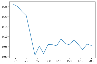
The line plot showing Silhouette scores at different numbers of clusters is shown below:

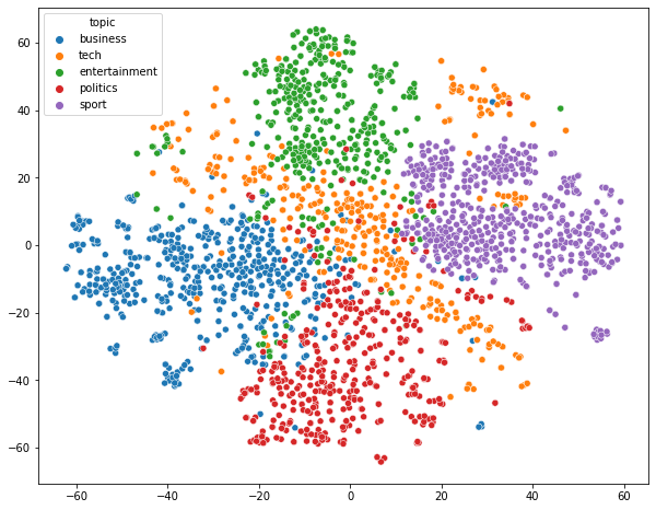
The plot shows clearly that the silhouette scores are quite low. Thus, either the clusters are not linearly separable or there is a considerable amount of overlaps among them. A TSNE plot is better suited in such a case. The TSNE plot extracts a low dimensional representation of high dimensional data through a non-linear embedding method which tries to retain the local structure of the data. The code as well as the TSNE plot is shown below.

tsne = TSNE(n_components=2)
tsne_mat = tsne.fit_transform(tsvd_mat)

plt.figure(figsize=(10,8))
sns.scatterplot(tsne_mat[:,0],tsne_mat[:,1],hue=df_final['topic'])

In this plot, only the tech-related news article looks like having a much wider spread whereas other news articles look quite nicely clustered. It also suggests that LSA (or Truncated SVD) has done a good job on the textual data to extract 200 important dimensions to segregate news articles on different topics. It is to be understood that TSNE is non-deterministic in nature and multiple runs will produce multiple representations, even though, the structure will be more likely to remain similar if not the same. This LSA can be also used for text queries, for example,

from sklearn.metrics import pairwise_distances
import numpy as np
query = "How is Microsoft performing in computer game?"
query_mat = tsvd.transform(dtm.transform([query]))
dist = pairwise_distances(X=tsvd_mat, Y=query_mat, metric='cosine')
df_final['News'][np.argmin(dist.flatten())]