Maximum Likelihood Estimation

The purpose of this guide is to explore the idea of Maximum Likelihood Estimation, which is perhaps the most important concept in Statistics. If you’re interested in familiarizing yourself with the mathematics behind Data Science, then maximum likelihood estimation is something you can’t miss. For most statisticians, it’s like the sine qua non of their discipline, something without which statistics would lose a lot of its power.Also , in this article you will get concepts of maximum likelihood method of estimation, how maximum likelihood function, maximum likelihood and how do maximum likelihood estimators (mle) work? i.e mle likelihood get a proper understanding.

This article was published as a part of the Data Science Blogathon

What is Maximum Likelihood Estimation (MLE)?

Maximum Likelihood Estimation (MLE) is a statistical technique used to estimate the parameters of a model by finding the values that make the observed data most probable. It works by calculating the likelihood, which measures how well the model explains the data for a given set of parameters. MLE seeks the parameter values that maximize this likelihood, effectively identifying the most plausible estimates based on the data. For example, if flipping a coin results in 7 heads out of 10 flips, MLE would estimate the probability of heads as 0.7, as this value best explains the observed outcome.

Mle likelihood

Estimators are tools that use your data to estimate the values of parameters you’re interested in. Common examples include the sample mean (used to estimate the average of a distribution) and the sample variance (used to estimate the spread of a distribution). While it might seem logical to use estimators that match the parameter’s role (like using the sample mean for the average), this approach has limitations.

1) Things aren’t always that simple. Sometimes, you may encounter problems involving estimating parameters that do not have a simple one-to-one correspondence with common numerical characteristics. For instance, if I give you the following distribution:

The above equation shows the probability density function of a Pareto distribution with scale=1. It’s not easy to estimate parameter θ of the distribution using simple estimators based because the numerical characteristics of the distribution vary as a function of the range of the parameter. For instance, the mean of the above distribution is expressed as follows:

This is just one example picked from the infinitely possible sophisticated statistical distributions. (We’ll later see how we can use the use Maximum Likelihood Estimation to find an apt estimator for the parameter θ of the above distribution)

2) Even if things were simple, there’s no guarantee that the natural estimator would be the best one. Sometimes, other estimators give you better estimates based on your data. In the 8^th section of this article, we would compute the MLE for a set of real numbers and see its accuracy.

This article explains maximum likelihood estimation (MLE), a method that creates powerful estimators called maximum likelihood estimators (MLEs). MLEs are considered highly effective. We’ll explore what MLEs are, how to find them, and why they’re useful.

Let’s start our journey into the magical and mystical realm of MLEs.

Pre-requisites:

• Probability: Basic ideas about random variables, mean, variance and probability distributions. If you’re unfamiliar with these ideas, then you can read one of my articles on ‘Understanding Random Variables.
• Mathematics: Preliminary knowledge in Calculus and Linear Algebra; ability to solve simple convex optimization problems by taking partial derivatives; calculating gradients.
• Passion: Finally, reading about something without having a passion for it is like knowing without learning. Real learning comes when you have a passion for the subject and the concept that is being taught.

Basics of Statistical Modelling for Maximum Likelihood Estimation

Statistical modelling is the process of creating a simplified model for the problem that we’re faced with. For us, it’s using the observable data we have to capture the truth or the reality (i.e., understanding those numerical characteristics). Of course, it’s not possible to capture or understand the complete truth. So, we will aim to grasp as much reality as possible.

In general, a statistical model for a random experiment is the pair:

There are a lot of new variables! Let’s understand them one by one.

Maximum Likelihood Method of Estimation

• E represents the sample space of an experiment. By experiment we mean the data that we’ve collected- the observable data. So, E’s the range of values that our data can take (based on the distribution that we’ve assigned to it).
• ℙ_θ represents the family of probability-measures on E. In other words, it indicates the probability distribution that we’ve assigned to our data (based on our observations).
• θ represents the set of unknown parameters that characterize the distribution ℙ_θ. All those numerical features we wish to estimate are represented by θ. For now, it’s enough to think of θ as a single parameter that we’re trying to estimate. We’ll later see how to deal with multi-dimensional parameters.
• Θ represents the parameter space i.e., the range or the set of all possible values that the parameter θ could take.

Let’s take 2 examples:

A) For Bernoulli Distribution: We know that if X is a Bernoulli random variable, then X can take only 2 possible values- 0 and 1. Thus, the sample space E is the set {0, 1}. The Bernoulli probability distribution is shown as Ber(p), where p is the Bernoulli parameter, which represents the mean or the probability of success. Since it’s a measure of probability, p always ranges between 0 and 1. Therefore, Θ = [0, 1]. Putting all of this together, we obtain the following statistical model for Bernoulli distribution:

B) For Exponential Distribution: We know that if X is an exponential random variable, then X can take any positive real value. Thus, the sample space E is [0, ∞). The exponential probability distribution is shown as Exp(λ), where λ is the exponential parameter, that represents the rate (here, the inverse mean). Since X is always positive, its expectation is always positive, and therefore the inverse-mean or λ is positive. Therefore, Θ = (0, ∞). Putting all of this together, we obtain the following statistical model for exponential distribution:

Hope you all have got a decent understanding of creating formal statistical models for our data. Most of this idea would be used only when we introduce formal definitions and go through certain examples. Once you get well versed in the process of constructing MLEs, you won’t have to go through all of this.

A Note on Notations: In general, the notation for estimators is a hat over the parameter we are trying to estimate i.e. if θ is the parameter we’re trying to estimate, then the estimator for θ is represented as θ-hat. We shall use the terms estimator and estimate (the value that the estimator gives) interchangeably throughout the guide.

Before proceeding to the next section, I find it important to discuss an important assumption that we shall make throughout this article- identifiability.

Identifiability means that different values of a parameter (from the parameter space Θ) must produce different probability distributions. In other words, for two different values of a parameter (θ & θ’), there must exist two different distributions (ℙ _θ & ℙ _θ’). That is,

Equivalently,

Total Variation Distance for Maximum Likelihood Estimation

Here, we’ll explore the idea of computing distance between two probability distributions. There could be two distributions from different families such as the exponential distribution and the uniform distribution or two distributions from the same family, but with different parameters such as Ber(0.2) and Ber(0.8). The notion of distance is commonly used in statistics and machine learning- finding distance between data points, the distance of a point from a hyperplane, the distance between two planes, etc.

How can we compute the distance between two probability distributions? One of the most commonly used metrics by statisticians is Total Variation (TV) Distance, which measures the worst deviation between two probability distributions for any subset of the sample space E.

Mathematically we define the total variation distance between two distributions ℙ and ℚ as
follows:

Intuitively, total variation distance between two distributions ℙ and ℚ refers to the maximum difference in their probabilities computed for any subset over the sample space for which they’re defined. To understand it better, let us assign random variables X and Y to ℙ and ℚ respectively. For all A that are subsets of E, we find ℙ(A) and ℚ(A), which represent the probability of X and Y taking a value in A. We find the absolute value of the difference between those probabilities for all A and compare them. The maximum absolute difference is the total variation distance. Let’s take an example.

Maximum Likelihood Function

Compute the total variation distance between ℙ and ℚ where the probability mass functions are as follows:

Since the observed values of the random variables corresponding to ℙ and ℚ are defined only over 1 and 2, the sample space is E = {1, 2}. What are the possible subsets? There are 3 possible subsets: {1}, {2} and {1, 2}. (We may always ignore the null set). Let’s compute the absolute difference in ℙ(A) and ℚ(A) for all possible subsets A. 

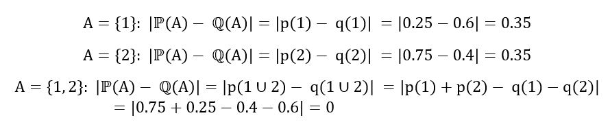
Therefore, we can compute the TV distance as follows:

That’s it. Suppose, we are now asked to compute TV distance between Exp(1) and Exp(2) distribution. Could you find the TV distance between them using the above method? Certainly not! Exponential distributions have E = [0, ∞). There will be infinite subsets of E. You can’t find ℙ(A) and ℚ(A) for each of those subsets. To deal with such situations, there’s a simpler analytical formula for the computation of TV Distance, which is defined differently depending on whether ℙ and ℚ are discrete or continuous distributions.

A) For the discrete case,

If ℙ and ℚ are discrete distributions with probability mass functions p(x) and q(x) and sample space E, then we can compute the TV distance between them using the following equation:

Let’s use the above formula to compute the TV distance between ℙ=Ber(α) and ℚ=Ber(β). The calculation is as follows:

E = {0,1} since we’re dealing with Bernoulli random variables.

Using the short-cut formula, we obtain,

That’s neater! Now, let’s talk about the continuous case.

B) For the continuous case,

If ℙ and ℚ are continuous distributions with probability density functions p(x) and q(x) and sample space E, then we can compute the TV distance between them using the following equation:

Let’s use the above formula to compute the TV distance between ℙ=Exp(1) and ℚ=Unif[0,1] (the uniform distribution between 0 and 1). The calculation is as follows:

We’ve used the indicator function 𝕀 above, which takes the value 1 if the condition in the curly brackets is satisfied and 0 otherwise. We could have also described the probability density functions without using the indicator function as follows:

The indicator functions make the calculations look neater and allow us to treat the entire real line as the sample space for the probability distributions.

Using the short-cut formula, we obtain,

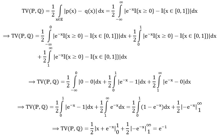
Thus, we’ve obtained the required value. (Even imagining doing this calculation without the analytical equation seems impossible).

We shall now see some mathematical properties of Total Variation Distance:

• Symmetry

• Definiteness

• Range

• Triangle Inequality

That almost concludes our discussion on TV distance. You might be wondering about the reason for this detour. We started our discussion with MLE and went on to talk about TV distance. What’s the connection between them? Are they related to each other? Well, technically no. MLE is not based on TV distance, rather it’s based on something called as Kullback-Leibler divergence, which we’ll see in the next section. But an understanding of TV distance is still important to understand the idea of MLEs.

This guide now focuses on a key and challenging step: building an estimator using TV distance. To do this, we’ll use a property of TV distance called definiteness, which shows the value TV distance approaches as two distributions become identical. We’ll examine two distributions from the same family but with different parameters.

ℙ_θ and ℙ_θ*, where θ is the parameter that we are trying to estimate, θ* is the true value of the parameter θ and ℙ is the probability distribution of the observable data we have. From definiteness, we have,

(Notice how the above equation has used identifiability). Since we had also learnt that the minimum value of TV distance is 0, we can also say:

Graphically, we may represent the same as follows:

(The blue curve could be any function that ranges between 0 and 1 and attains minimum value = 0 at θ*). It will not be possible for us to compute the function TV(ℙ_θ, ℙ_θ*) in the absence of the true parameter value θ*. What if we could estimate the TV distance and let our estimator be the minimizer of the estimated TV distance between ℙ_θ and ℙ_θ*?!

In estimation, our goal is to find an estimator θ-hat for the parameter θ such that θ-hat is close to the true parameter θ*. We can see that in terms of minimizing the distance between the distributions ℙ_θ and ℙ_θ*. And that’s when TV distance comes into the picture. We want an estimator θ-hat such that when θ = θ-hat, the estimated TV distance between the probability measures under θ and θ* is minimized. That is, θ =θ-hat should be the minimizer of the estimated TV distance between ℙ_θ and ℙ_θ*. Mathematically, we can describe θ-hat as:

Graphically,

Kullback-Leibler Divergence

KL divergence, also known as relative entropy, like TV distance is defined differently depending on whether ℙ and ℚ are discrete or continuous distributions.

• For the discrete case : If ℙ and ℚ are discrete distributions with probability mass functions p(x) and q(x) and sample space E, then we can compute the KL divergence between them using the following equation:

The equation certainly looks more complex than the one for TV distance, but it’s more amenable to estimation. We’ll see this later in this section when we talk about the properties of KL divergence.

Let’s use the above formula to compute the KL divergence between ℙ=Ber(α) and ℚ=Ber(β). The calculation is as follows:

Using the formula, we obtain,

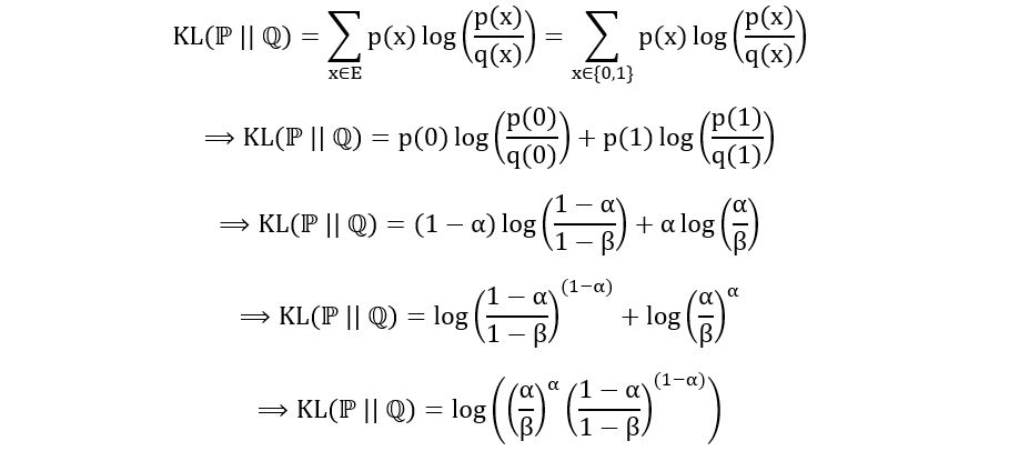
That’s it. A more difficult computation, but we’ll see its utility later.

• For the continuous case : If ℙ and ℚ are continuous distributions with probability density functions p(x) and q(x) and sample space E, then we can compute the KL divergence between them using the following equation:

Let’s use the above formula to compute the KL divergence between ℙ=Exp(α) and ℚ=Exp(β). The calculation is as follows:

Since we’re dealing with exponential distributions, the sample space E is [0, ∞). Using the formula, we obtain,

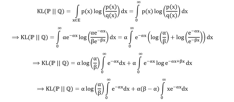
Don’t worry, I won’t make you go through the long integration by parts to solve the above integral. Just use wolfram or any integral calculator to solve it, which gives us the following result:

And we’re done. That’s how we can compute the KL divergence between two distributions. If you’d like to practice more, try computing the KL divergence between ℙ=N(α, 1) and ℚ=N(β, 1) (normal distributions with different mean and same variance). Let me know your answers in the comment section.

We now explore the properties of KL divergence, which differ from TV distance as it is a divergence, not a distance. Unlike distances, KL divergence lacks symmetry and the triangle inequality, but it maintains definiteness, enabling estimator construction. Note: we focus on continuous distributions; for discrete cases, replace integrals with sums. Below are the key properties of KL divergence:

1) Asymmetry (in general):

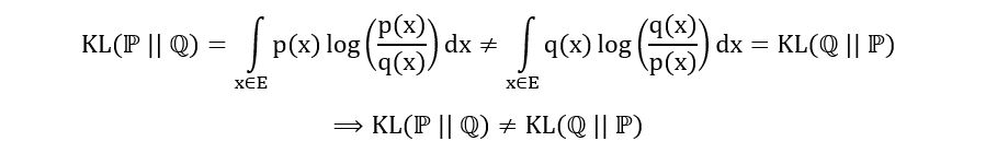
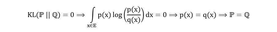
2) Definiteness:

3) Range:

(Yes, KL divergence can be greater than one because it does not represent a probability or a difference in probabilities. The KL divergence also goes to infinity for some very common distributions such as the KL divergence between two uniform distributions under certain conditions)

4) No Triangle Inequality (in general):

5) Amenable to Estimation:

Recall, the properties of expectation: If X is a random variable with probability density function f(x) and sample space E, then

If we replace x with a function of x, say g(x), we get

We’ve used just this in the expression for KL divergence. The probability density function is p(x) and g(x) is log(p(x)/q(x)). We’ve also put a subscript x~ℙ to show that we’re calculating the expectation under p(x). So we have,

We’ll see how this makes KL divergence estimable in section 4. Now, let’s use the ideas discussed at end of section 2 to address our problem of finding an estimator θ-hat to parameter θ of a probability distribution ℙ_θ:

We consider the following two distributions (from the same family, but different parameters):

ℙ_θ and ℙ_θ*, where θ is the parameter that we are trying to estimate, θ* is the true value of the parameter θ and ℙ is the probability distribution of the observable data we have.

From definiteness, we have,

(Notice how the above equation has used identifiability). Since we had also learnt that the minimum value of KL divergence is 0, we can say:

Graphically, we may represent the same as follows:

(The blue curve could be any function that ranges between 0 and infinity and attains minimum value = 0 at θ*). It will not be possible for us to compute the function KL(ℙ_θ* || ℙ_θ) in the absence of the true parameter value θ*. So, we estimate it and let our estimator θ-hat be the minimizer of the estimated KL divergence between ℙ_θ* and ℙ_θ.

Mathematically, 

And that estimator is precisely the maximum likelihood estimator. We’ll simplify the above expression in the next section and understand the reasoning behind its terminology.

Graphically,

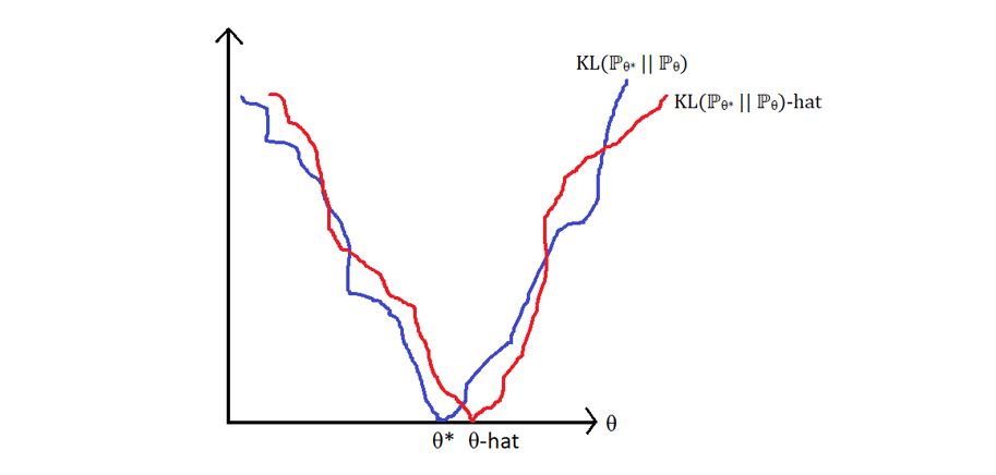
Image by Author

We want to be able to estimate the blue curve (KL(ℙ_θ* || ℙ_θ)) to find the red curve (KL(ℙ_θ* || ℙ_θ)-hat). The value of θ that minimizes the red curve would be θ-hat which should be close to the value of θ that minimizes the blue curve i.e., θ*. And the best part is, unlike TV distance, we can estimate KL divergence and use its minimizer as our estimator for θ.

That’s how we get the MLE.

Deriving the Estimator fo Maximum Likelihood Estimation

In the previous section, we obtained that the MLE θ-hat is calculated as:

We have considered the distributions ℙ_θ and ℙ_θ*, where θ is the parameter that we are trying to estimate, θ* is the true value of the parameter θ and ℙ is the probability distribution of the observable data we have. Let the probability distribution functions (could be density or mass depending upon the nature of the distribution) be p_θ(x) and p_θ*(x).

(Notice that we’ve used the same letter p to denote the distribution functions as both the distributions belong to the same family ℙ. Also, the parameter has been subscripted to distinguish the parameters under which we’re calculating the distribution functions.)

We have also shown the process of expressing the KL divergence as an expectation:

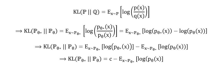
Where c =E_x~ℙθ*[log(p_θ*(x))] is treated as a constant as it is independent of θ. (θ* is a constant value). We won’t be needing this quantity at all as we want to minimize the KL divergence over θ.

So, we can say that,

How is this useful to us? Recall what the law of large numbers gives us. As our sample size (no. of observations) grows bigger, then the sample mean of the observations converges to the true mean or expectation of the underlying distribution. That is, if Y₁, Y₂, …, Y_n are independent and identically distributed random variables, then

We can replace Y_i with any function of a random variable, say log(p_θ(x)). So, we get, 

Thus, using our data, we can find the 1/n*sum(log(p_θ(x)) and use that as an estimator for E_x~ℙθ*[log(p_θ(x))]

Thus, we have, 

Substituting this in equation 2, we obtain:

Finally, we’ve obtained an estimator for the KL divergence. We can substitute this in equation 1, to obtain the maximum likelihood estimator:

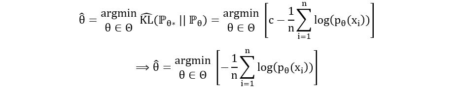
(Addition of a constant can only shift the function up and down, not affect the minimizer of the function)

(Finding the minimizer of negative of f(x) is equivalent to finding the maximizer of f(x))

(Multiplication of a function by a constant does not affect its maximize)

(log(x) is an increasing function, the maximizer of g(f(x)) is the maximizer of f(x) if g is an increasing function)

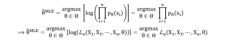
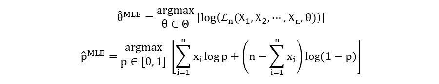
Thus, the maximum likelihood estimator θ^MLE-hat (change in notation) is defined mathematically as:

П(p_θ(x_i)) is called the likelihood function. Thus, the MLE is an estimator that is the maximizer of the likelihood function. Therefore, it is called the Maximum Likelihood Estimator. We’ll understand the likelihood function in greater detail in the next section.

Understanding and Computing the Maximum Likelihood Estimation Function

The likelihood function is defined as follows:

• For discrete case: If X₁, X₂, …, X_n are identically distributed random variables with the statistical model (E, {ℙ_θ}_θ∈Θ), where E is a discrete sample space, then the likelihood function is defined as:

Furthermore, if X₁, X₂, …, X_n are independent,

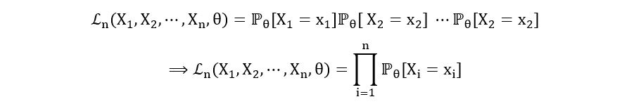
By definition of probability mass function, if X₁, X₂, …, X_n have probability mass function p_θ(x), then, ℙ_θ[X_i=x_i] = p_θ(x_i). So, we have:

• For continuous case: It’s the same as before. We just need to replace the probability mass function with the probability density function. If X₁, X₂, …, X_n are independent and identically distributed random variables with the statistical model (E, {ℙ_θ}_θ∈Θ), where E is a continuous sample space, then the likelihood function is defined as:

Where, p_θ(x_i) is the probability density function of the distribution that X₁, X₂, …, X_n follow.

To better understand the likelihood function, we’ll take some examples.

• Bernoulli Distribution:

Model:

Parameter: θ=p

Probability Mass Function:

Likelihood Function:

• Poisson Distribution:

Model:

(Sample space is the set of all whole numbers)

Parameter: θ=λ

Probability Mass Function:

Likelihood Function:

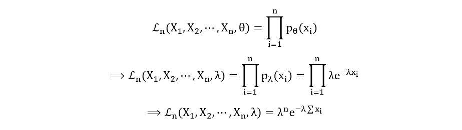
• Exponential Distribution:

Model:

Parameter: θ=λ

Probability Density Function:

Likelihood Function:

• Uniform Distribution: This one’s also going to be very interesting because the probability density function is defined only over a particular range, which itself depends upon the value of the parameter to be estimated.

Model:

Parameter: θ=α

Probability Density Function:

(We can ignore the part where x should be more than 0 as it is independent of the parameter α)

Likelihood Function:

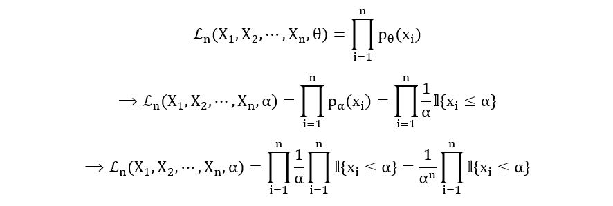
That seems tricky. How should we take the product of indicator functions? Remember, the indicator function can take only 2 values- 1 (if the condition in the curly brackets is satisfied) and 0 (if the condition in the curly brackets is not satisfied). If all the x_i’s satisfy the condition under the curly brackets, then the product of the indicator functions will also be one. But if even one of the x_i’s fails to satisfy the condition, the product will become zero. Therefore, the product of these indicator functions itself can be considered as an indicator function that can take only 2 values- 1 (if the condition in the curly brackets is satisfied by all x_i’s) and 0 (if the condition in the curly brackets is not satisfied by at least 1 x_i). Therefore,

(All x_i’s are less than α if and only if max{x_i} is less than α)

And this concludes our discussion on likelihood functions. Hope you had fun practicing these problems!

What are the advantages of using maximum likelihood over maximum probability?

Here are some additional advantages of using maximum likelihood over maximum probability:

• MLE is more consistent. This means that if we were to repeat the estimation procedure many times, using different samples of data, the MLE would eventually converge to the true value of the parameter.
• MLE is more asymptotically efficient. This means that as the sample size increases, the MLE becomes more and more accurate.
• MLE is more versatile. It can be used to estimate the parameters of a wide variety of statistical models, including both parametric and non-parametric models.

Overall, maximum likelihood estimation is a powerful and versatile method for statistical inference. It is a good choice for many situations, especially when the data is abundant and reliable.

Computing the Maximum Likelihood Estimator for Single-Dimensional Parameters

In this section, we’ll use the likelihood functions computed earlier to obtain the maximum likelihood estimators for some common distributions. This section will be heavily reliant on using tools of optimization, primarily first derivative test, second derivative tests, and so on. We won’t go into very complex calculus in this section and will restrict ourselves to single variable calculus. Multivariable calculus would be used in the next section.

Earlier on, we had obtained the maximum likelihood estimator which is defined as follows:

We also saw that П(p_θ(x_i)) was the likelihood function. The MLE is just the θ that maximizes the likelihood function. So our job is quite simple- just maximize the likelihood functions we computed earlier using differentiation.

Note: Sometimes differentiating the likelihood function isn’t easy. So, we often use log-likelihood instead of likelihood. Using logarithmic functions saves us from using the notorious product and division rules of differentiation. Since log(x) is an increasing function, the maximizer of log-likelihood and likelihood is the same.

Examples:

To better understand the likelihood function, we’ll take some examples.

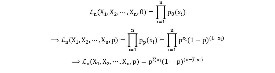
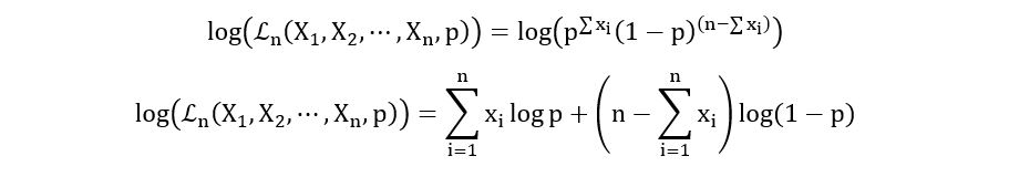
I) Bernoulli Distribution:

Likelihood Function:

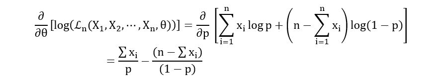
Log-likelihood Function:

Maximum Likelihood Estimator:

Calculation of the First derivative:

Calculation of Critical Points in (0, 1)

Calculation of the Second derivative:

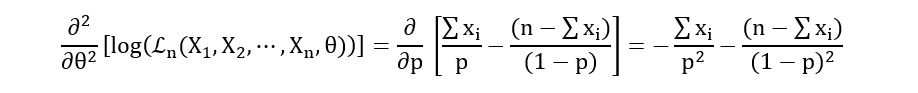
Substituting equation 6.1 in the above expression, we obtain,

Therefore, p = 1/n*(sum(x_i)) is the maximizer of the log-likelihood. Therefore,

The MLE is the sample-mean estimator for the Bernoulli distribution! Yes, the one we talked about at the beginning of the article. Isn’t it amazing how something so natural as the mean could be produced using rigorous mathematical formulation and computation!

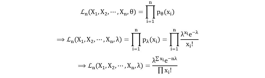
II) Poisson Distribution:

Likelihood Function:

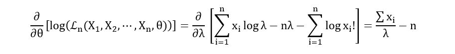
Log-likelihood Function:

Maximum Likelihood Estimator:

Calculation of the First derivative:

Critical Points in (0, ∞)

Second derivative:

Substituting equation 6.2 in the above expression, we obtain,

Therefore, λ = 1/n*(sum(x_i)) is the maximizer of the log-likelihood. Thus,

It’s again the sample-mean estimator!

III) Exponential Distribution:

Likelihood Function:

Log-likelihood Function:

Maximum Likelihood Estimator:

First derivative:

Points in (0, ∞)

Second derivative:

Substituting equation 6.3 in the above expression, we obtain,

Therefore, λ = (sum(x_i))/n is the maximizer of the log-likelihood. Therefore,

IV) Uniform Distribution:

Likelihood Function:

Here, we don’t need to use the log-likelihood function. Nor do we have to use the tools of calculus. We’ll try to find the maximizer of the above likelihood function using pure logic. We have, 

Since n represents the sample size, n is positive. Therefore, for constant n, the likelihood increases as α decreases. The likelihood function would be maximized for the minimum value of α. What’s the minimum value? It’s not zero. See the expression inside the curly brackets. 

Therefore, the minimum value of α is max{x_i}. Thus,

This concludes our discussion on computing the maximum likelihood
estimator for statistical models with single parameters.

Computing the Maximum Likelihood Estimator for Multi-Dimensional Parameters

In this section, we’ll use the likelihood functions computed earlier to obtain the maximum likelihood estimators for the normal distributions, which is a two-parameter model. This section would require familiarity with basic instruments of multivariable calculus such as calculating gradients. If you find yourself unfamiliar with these tools, don’t worry! You may choose to ignore the mathematical intricacies and understand only the broad idea behind the computations. We’ll use all those tools only for optimizing the multidimensional functions, which you can easily do using modern calculators.

The problem we wish to address in this section is finding the MLE for a distribution that is characterized by two parameters. Since normal distributions are the most famous in this regard, we’ll go through the process of finding MLEs for the two parameters- mean (µ) and variance (σ²). The process goes as follows:

Statistical Model:

E = (-∞, ∞) as a gaussian random variable can take any value on the real line.

θ = (µ, σ²) is interpreted as a 2-dimensional parameter (Intuitively think of it as a set of 2 parameters).

Θ = (-∞, ∞) × (0, ∞) as mean (µ) can take any value in the real line and variance (σ²) is always positive.

Parameter: θ = (µ, σ²)

Probability Density Function:

Likelihood Function:

Log-likelihood Function:

We now maximize the above multi-dimensional function as follows:

Computing the Gradient of the Log-likelihood:

Setting the gradient equal to the zero vector, we obtain,

On comparing the first element, we obtain:

On comparing the second element, we obtain:

Thus, we have obtained the maximum likelihood estimators for the parameters of the gaussian distribution:

The estimator for variance is popularly called the biased sample variance estimator.

Demystifying the Pareto Problem w.r.t. Maximum Likelihood Estimation

One of the probability distributions that we encountered at the beginning of this guide was the Pareto distribution. Since there was no one-to-one correspondence of the parameter θ of the Pareto distribution with a numerical characteristic such as mean or variance, we could not find a natural estimator. Now that we’re equipped with the tools of maximum likelihood estimation, let’s use them to find the MLE for the parameter θ of the Pareto distribution. Recall that the Pareto distribution has the following probability density function:

Graphically, it may be represented as follows (for θ=1):

• Model:

(Shape parameter (θ) is always positive. The sample space must be greater than the scale, which is 1 in our case)

• Parameter: θ

• Probability Density Function:

• Likelihood Function:

• Log-likelihood Function:

• Maximum Likelihood Estimator:

• Calculation of the First derivative:

• Calculation of Critical Points in (0, ∞)

• Calculation of the Second derivative:

Substituting equation 8.1 in the above expression, we obtain,

• Result:

Therefore, θ = n/(sum(log(x_i))) is the maximizer of the log likelihood. Therefore,

To make things more meaningful, let’s plug in some real numbers. We’ll be using R to do the calculations.

I’ve randomly generated the following set of 50 numbers from a Pareto distribution with shape (θ)=scale=1 using the following R code:

install.packages(‘extremefit’)
library(extremefit)
xi<-rpareto(50, 1, 0, 1)

The first argument (50) shows the sample size. The second argument (1) shows the shape parameter (θ). You may ignore the third argument (it shows the location parameter, which is set to zero by default). The fourth argument (1) shows the scale parameter, which is set to 1. The following set of numbers was generated:

Let’s evaluate the performance of our MLE. We should expect the MLE to be close to 1 to show that it’s a good estimator. Calculations:

n=50
S<-sum(log(xi))
MLE<-n/S

Output: 1.007471

That’s incredibly close to 1! Indeed, the MLE is doing a great job. Go ahead, try changing the sample sizes, and calculating the MLE for different samples. You can also try changing the shape parameter or even experiment with other distributions.

How do maximum likelihood estimators (mle) work?

Select a probability distribution that precisely depicts your data. This might be a common distribution, binomial distribution, Poisson distribution, or another appropriate distribution.

• Create the Probability of Event Function: This function shows the chance of coming across the specified data, based on the selected probability distribution and its parameters. It basically originates from the probability density functions (PDFs) of every data point.
• Enhance the Probability: The goal is to discover the parameter values that optimize the probability function. Frequently, this involves taking the logarithm of the likelihood function (log-likelihood) in order to make the computations easier.

Identify parameter values that optimize the log-likelihood function for calculating maximum likelihood estimates (MLEs).

Example:

Tossing a coin.

Picture tossing a coin 10 times and realizing that you see 7 heads. You need to calculate the likelihood of getting a heads result (p).

Probability distribution: Distribution characterized by its Binomial nature.

The formula for probability can be written as P(p) = p to the power of 7 multiplied by (1-p) to the power of 3.

To maximize likelihood, we can utilize the logarithm and obtain log L(p) = 7log(p) + 3log(1-p). When we set the derivative to zero with respect to p, we determine that the value of p is 0.7.

The MLE indicates a probability of 0.7 for obtaining heads.

Conclusion

The purpose of this article was to see MLEs not as abstract functions, but as mesmerizing mathematical constructs that have their roots deeply seated under solid logical and conceptual foundations. I hope you enjoyed going through this guide!

Hope you like the article and get clear understanding of maximum likelihood estimation covering the topics maximum likelihood method of estimation , mle likelihood and maximum likelihood function we are covering these topics . Hope you will assure and like the article.

Frequently Asked Questions