This article was published as a part of the Data Science Blogathon
Introduction
Hello everyone, in this article we will pick the use case of sequence modelling, which is time series forecasting. Time series is all around us from predicting sales to predicting traffic and more.
A simple example of time series is the amount of year-on-year passenger traffic in the U.S. Formally, time series is just a series of data points arranged in time order or in sequence commonly taken us successive, equally spaced points time.
Time-series Database is the fastest-growing category of databases in the past two years, and both traditional and emerging technology industries have been generating more and more time-series data.
Now let’s try to understand the business use case that we tackling here.
The web traffic is basically the number of sessions in a given time frame, and it varies a lot with respect to what time of the day it is, what day of the week it is, and so on, and how much web traffic of platform can withstand depends on the size of the servers that are supporting the platform.
If the traffic is more than what the servers can handle, the website might show this 404 error, which is something we don’t want to happen. It will make the visitors go away.
One solution to this problem is to increase the number of servers. However, the downside of the solution is the cause can go up, which is again undesirable. So, what is the solution?
You can dynamically a lot of servers based on the historical visitor’s volume data or based on the historical web traffic data. And that brings us to the data science problem, which is basically forecasting the web traffic or a number of sessions based on the historical data.
We will deep dive into the web traffic data set and look at how we can use LSTM to solve this time series forecasting problem.
Now we will cover the problem statement of web traffic forecasting, and how it will help in scaling the resources, backing the outline publishing platform.
We will work with the web traffic dataset. It is a six-month series data set the link is given here Link.
Load Dataset for Web Traffic Forecasting
Here we are reading the dataset by using pandas. It has over 4800 observations.
import pandas as pd
import numpy as np
data=pd.read_csv('webtraffic.csv')
Check the shape of the data
data.shape

To print the first records of the dataset.
data.head()
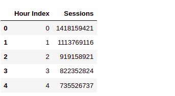
The first column is the hours as in this is the first hours, this is the second hour and so on.
And the second column session is the volume of traffic at an hourly level.
For example:- this is the number of sessions in the second hours and so on.
Data Exploration for Web Traffic Forecasting
Now let’s explore the data, we will use the below code to plot the entire time series there you go.
import matplotlib.pyplot as plt
sessions = data['Sessions'].values
ar = np.arange(len(sessions))
plt.figure(figsize=(22,10))
plt.plot(ar, sessions,'r')
plt.show()
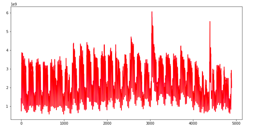
Each point of this curve is an early session count and you can see there are some repeating patterns throughout the time series.
The traffic volume comes down, after almost equal intervals of time. Apart from that, there are a couple of spikes as well in the traffic, In this plot.
Let’s explore this data, at a more granular level, we can use the below code and replace the entire time series, with a subset of it.
#first week web traffic
sample = sessions[:168]
ar = np.arange(len(sample))
plt.figure(figsize=(22,10))
plt.plot(ar, sample,'r')
plt.show()
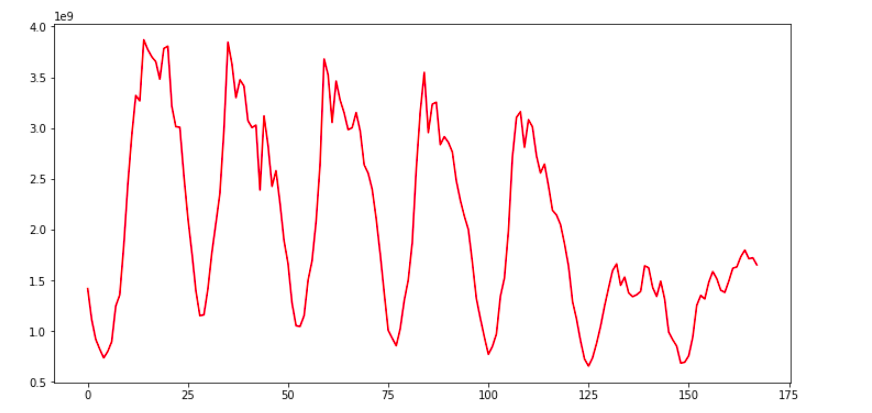
Here we are plotting the first week’s data only, now the repeating pattern can be seen more clearly, and these dips in the plot in web traffic are may be occurring once every 24 hours. So clearly there are two instances of time in a day, when we have a huge traffic volume, like during a few times and when we have a modest level of traffic on the website. As in here, I will help you to explore this data as much as possible, before getting started with model building.
Data Preparation for Web Traffic Forecasting
Moving on now let’s prepare the data for model training, here we will create input sequences, from the block traffic data. Let’s say this is a time series. Each cell would have some number or value. Let’s create sequences of length five, so the first five observations, will form the first sequence, and the sixth observation, this one will be treated as the target.
The second sequence will start from the second element, till the sixth element and the target will be the seventh element.


Now the subsequent sequences will be extracted, by moving this window, one step at a time.
def prepare_data(seq,num):
  x=[]
  y=[]
  for i in range(0,(len(seq)-num),1):

    input_ = seq[i:i+num]
    output  = seq[i+num]

    x.append(input_)
    y.append(output)

  return np.array(x), np.array(y)
In this function, prepare_data. We are using the same technique to create sequences from time-series data. We have specified the sequence length of one week or 168 hours.
num=168
x,y= prepare_data(sessions,num)
print(len(x))
Now here we are calling this function to create sequences. The sequence length we have specified is 168 hours and that is equivalent to one week. So we are creating sequences of one week, as our input sequences. Now the number of sequences are well over 4700.
Split the Dataset
Next, we have to split the data into a training set and validation set and we will do this in the ratio, 90 is to 10. Now that sense it is a time serious problem, we are not splitting the data randomly, we are splitting it in a sequential manner. As you can see the code below.
ind = int(0.9 * len(x))
x_tr = x[:ind]
y_tr = y[:ind]
x_val=x[ind:]
y_val=y[ind:]
nowhere in the code we would scale the data, Both the input sequences and the target values, will be scaled because of scaling the data, speeds because of scaling the data, speeds of the model training process.
from sklearn.preprocessing import StandardScaler
#normalize the inputs
x_scaler= StandardScaler()
x_tr = x_scaler.fit_transform(x_tr)
x_val= x_scaler.transform(x_val)
#reshaping the output for normalization
y_tr=y_tr.reshape(len(y_tr),1)
y_val=y_val.reshape(len(y_val),1)
#normalize the output
y_scaler=StandardScaler()
y_tr = y_scaler.fit_transform(y_tr)[:,0]
y_val = y_scaler.transform(y_val)[:,0]
After that, we are reshaping the data from two dimensional to 3 dimensional.
#reshaping input data
x_tr= x_tr.reshape(x_tr.shape[0],x_tr.shape[1],1)
x_val= x_val.reshape(x_val.shape[0],x_val.shape[1],1)
print(x_tr.shape)

The first dimension of our data is the number of sequences, and the second dimension is the number of elements in the sequences. But LSTM layer accepts only three-dimensional data.

These three dimensions are the number of sequences number of time steps and the length of the features. So third dimension is the length of the vectors of the sequence elements.
Let’s say I have five elements in my sequence and each of these elements has a vector length of 10. So this third dimension will become 10. If you can recall in the case of the auto-tagging projects the length of the sequence elements was nothing but the length of the word embeddings.
However in this dataset, the sequence elements are real number values and therefore the feature length is just one, hence we would reshape both the training set and the validation set as shown in the above code. Now, the data is ready for model training.
In the next section, we will build our deep learning model to predict traffic using LSTM.
Model Building for Web Traffic Forecasting
In the previous section, we covered how time-series data is converted into sequences to train data.
And now we will use these sequences to train a deep learning model to predict future web traffic. The first thing that we do is define the model architecture.
from keras.models import *
from keras.layers import *
from keras.callbacks import *
from tensorflow import keras
# define model
model =  Sequential()
model.add(LSTM(128,input_shape=(168,1)))
model.add(Dense(64,activation='relu'))
model.add(Dense(1,activation='linear'))
Have a look at the activation at the final layer above the code It is linear. This is because we have to predict a continuous value and not some class tag or category as it is a regression problem and not a classification problem. Other than that we are using a single layer of LSTM here and the input shape is 168 that is one week.
model.summary()
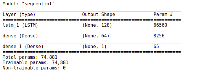
The number of train parameters is just around 74000.
# Define the optimizer and loss
model.compile(loss='mse',optimizer='adam')
#Define the callback to save the best model during the training
mc = ModelCheckpoint('best_model.hdf5', monitor='val_loss',
        verbose=1, save_best_only=True, mode='min')
# Train the model for 30 epochs with batch size of 32:
history=model.fit(x_tr, y_tr ,epochs=30, batch_size=32,
           validation_data=(x_val,y_val), callbacks=[mc])
The output will be:-
Epoch 1/30
133/133 [==============================] – 15s 101ms/step – loss: 0.1409 – val_loss: 0.0339Epoch 00001: val_loss improved from inf to 0.03390, saving model to best_model.hdf5
Epoch 2/30
133/133 [==============================] – 17s 126ms/step – loss: 0.0394 – val_loss: 0.0286Epoch 00002: val_loss improved from 0.03390 to 0.02865, saving model to best_model.hdf5
Epoch 3/30
133/133 [==============================] – 19s 142ms/step – loss: 0.0369 – val_loss: 0.0265Epoch 00003: val_loss improved from 0.02865 to 0.02647, saving model to best_model.hdf5
Epoch 4/30
133/133 [==============================] – 19s 142ms/step – loss: 0.0332 – val_loss: 0.0269Epoch 00004: val_loss did not improve from 0.02647
Epoch 5/30
133/133 [==============================] – 18s 137ms/step – loss: 0.0329 – val_loss: 0.0240Epoch 00005: val_loss improved from 0.02647 to 0.02402, saving model to best_model.hdf5
Epoch 6/30
133/133 [==============================] – 19s 143ms/step – loss: 0.0303 – val_loss: 0.0250Epoch 00006: val_loss did not improve from 0.02402
Epoch 7/30
133/133 [==============================] – 21s 155ms/step – loss: 0.0283 – val_loss: 0.0248Epoch 00007: val_loss did not improve from 0.02402
Epoch 8/30
133/133 [==============================] – 21s 156ms/step – loss: 0.0290 – val_loss: 0.0211Epoch 00008: val_loss improved from 0.02402 to 0.02107, saving model to best_model.hdf5
Epoch 9/30
133/133 [==============================] – 19s 146ms/step – loss: 0.0269 – val_loss: 0.0231Epoch 00009: val_loss did not improve from 0.02107
Epoch 10/30
133/133 [==============================] – 19s 140ms/step – loss: 0.0269 – val_loss: 0.0241Epoch 00010: val_loss did not improve from 0.02107
Epoch 11/30
133/133 [==============================] – 18s 138ms/step – loss: 0.0252 – val_loss: 0.0201Epoch 00011: val_loss improved from 0.02107 to 0.02014, saving model to best_model.hdf5
Epoch 12/30
133/133 [==============================] – 19s 144ms/step – loss: 0.0237 – val_loss: 0.0199Epoch 00012: val_loss improved from 0.02014 to 0.01994, saving model to best_model.hdf5
Epoch 13/30
133/133 [==============================] – 27s 201ms/step – loss: 0.0215 – val_loss: 0.0160Epoch 00013: val_loss improved from 0.01994 to 0.01602, saving model to best_model.hdf5
Epoch 14/30
133/133 [==============================] – 23s 170ms/step – loss: 0.0197 – val_loss: 0.0202Epoch 00014: val_loss did not improve from 0.01602
Epoch 15/30
133/133 [==============================] – 17s 127ms/step – loss: 0.0188 – val_loss: 0.0168Epoch 00015: val_loss did not improve from 0.01602
Epoch 16/30
133/133 [==============================] – 17s 127ms/step – loss: 0.0179 – val_loss: 0.0173Epoch 00016: val_loss did not improve from 0.01602
Epoch 17/30
133/133 [==============================] – 17s 125ms/step – loss: 0.0179 – val_loss: 0.0188Epoch 00017: val_loss did not improve from 0.01602
Epoch 18/30
133/133 [==============================] – 17s 127ms/step – loss: 0.0171 – val_loss: 0.0140Epoch 00018: val_loss improved from 0.01602 to 0.01395, saving model to best_model.hdf5
Epoch 19/30
133/133 [==============================] – 18s 133ms/step – loss: 0.0165 – val_loss: 0.0155Epoch 00019: val_loss did not improve from 0.01395
Epoch 20/30
133/133 [==============================] – 17s 127ms/step – loss: 0.0165 – val_loss: 0.0216Epoch 00020: val_loss did not improve from 0.01395
Epoch 21/30
133/133 [==============================] – 17s 126ms/step – loss: 0.0160 – val_loss: 0.0166Epoch 00021: val_loss did not improve from 0.01395
Epoch 22/30
133/133 [==============================] – 17s 125ms/step – loss: 0.0165 – val_loss: 0.0158Epoch 00022: val_loss did not improve from 0.01395
Epoch 23/30
133/133 [==============================] – 17s 126ms/step – loss: 0.0161 – val_loss: 0.0166Epoch 00023: val_loss did not improve from 0.01395
Epoch 24/30
133/133 [==============================] – 17s 128ms/step – loss: 0.0158 – val_loss: 0.0150Epoch 00024: val_loss did not improve from 0.01395
Epoch 25/30
133/133 [==============================] – 17s 127ms/step – loss: 0.0164 – val_loss: 0.0164Epoch 00025: val_loss did not improve from 0.01395
Epoch 26/30
133/133 [==============================] – 17s 131ms/step – loss: 0.0158 – val_loss: 0.0179Epoch 00026: val_loss did not improve from 0.01395
Epoch 27/30
133/133 [==============================] – 17s 127ms/step – loss: 0.0155 – val_loss: 0.0159Epoch 00027: val_loss did not improve from 0.01395
Epoch 28/30
133/133 [==============================] – 17s 127ms/step – loss: 0.0153 – val_loss: 0.0141Epoch 00028: val_loss did not improve from 0.01395
Epoch 29/30
133/133 [==============================] – 17s 128ms/step – loss: 0.0149 – val_loss: 0.0260Epoch 00029: val_loss did not improve from 0.01395
Epoch 30/30
133/133 [==============================] – 17s 128ms/step – loss: 0.0154 – val_loss: 0.0145Epoch 00030: val_loss did not improve from 0.01395
Load the weights of the best model prior to predictions. Now here we will use the mean squared error and we are using model checkpoint again to save the best model weight.
model.load_weights('best_model.hdf5')
finally, the model training starts and moving on the evaluation starts here and moving on to the evaluation part, the mean squared error for the validation data is just 0.013. Evaluate the performance of the model on the validation data.
mse = model.evaluate(x_val,y_val)
print("Mean Square Error:",mse)

Now, whenever we are working on a project it is always a good practice to have a baseline model, just to have an idea of how good your model is with respect to the baseline predictions.
Baseline Model with Forecasting
So here we are using a simple moving average as the baseline model. So what we will do, we will take a sequence and its length is the same 168 elements. And then we take average this sequence and we compare this average with the target value.
# build a simple moving average model
def compute_moving_average(data):
  pred=[]
  for i in data:
    avg=np.sum(i)/len(i)
    pred.append(avg)
  return np.array(pred)
# reshape the data
x_reshaped = x_val.reshape(-1,168)
# get predictions
y_pred = compute_moving_average(x_reshaped)
So this function computes the average of the input sequences and over here we are extracting the predictions.
# evaluate the performance of model on the validation data
mse = np.sum ( (y_val - y_pred) **2 ) / (len(y_val))
print("Mean square of error:- ",mse)
Now we calculate the mean squared error for this model. On the same validation data, we get a score of 0.554 which is way higher than this previous error.

So our LSTM based model has done exceptionally well as compared to the baseline model,
Web Traffic Forecasting
Now moving on to forecasting. These are the steps that we will follow:-
-
first, initialize an array with weeks data,
-
Predict the next hour traffic volume
-
Append the predicted value at the end of the array ‘data
-
Skip the first element of the array ‘data’
-
Repeating steps, from the second step till the fourth step for the specified number of iterations.
This is how we can forecasting for any number of hours in future. This function forecast performs the steps just discuss and it returns the predicted sequence of numbers.
def forecast(x_val, no_of_pred, ind):
  predictions=[]
  #intialize the array with a weeks data
  temp=x_val[ind]
for i in range(no_of_pred):
    #predict for the next hour
    pred=model.predict(temp.reshape(1,-1,1))[0][0]

    #append the prediction as the last element of array
    temp = np.insert(temp,len(temp),pred)
    predictions.append(pred)
    #ignore the first element of array
    temp = temp[1:]
return predictions
It’s time to forecast the traffic for the next 24 hours based on the previous week data.
no_of_pred =24
ind=72
y_pred= forecast(x_val,no_of_pred,ind)
y_true = y_val[ind:ind+(no_of_pred)]
# Lets convert back the normalized values to the original dimensional space
y_true= y_scaler.inverse_transform(y_true)
y_pred= y_scaler.inverse_transform(y_pred)
Now let’s look at the plot of real vs forecast values.
def plot(y_true,y_pred):
  ar = np.arange(len(y_true))
  plt.figure(figsize=(22,10))
  plt.plot(ar, y_true,'r')
  plt.plot(ar, y_pred,'y')
  plt.show()
plot(y_true,y_pred)
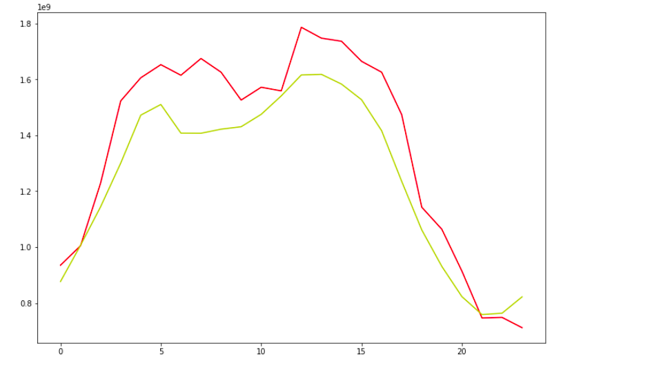
It looks great. Our model has been successful in capturing the trend.
This red curve is the actual value and this yellow curve are the predicted values both are pretty much close to each other.
Similarly, we can use a CNN based model in place of LSTM to perform the same task. Let’s see how it is done.
CNN Model with Forecasting
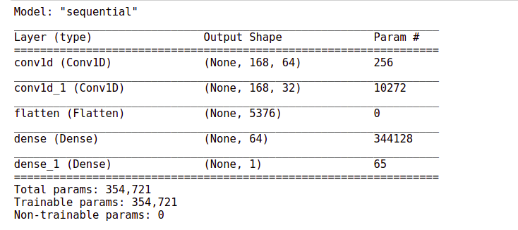
Now here we are using Conv1D layers in the model architecture. And these layers are followed by a flattening layer. This layer converts the input to a One Dimensional array, which is then passed on to this set of dense layers.
from tensorflow.keras.models import Sequential
from tensorflow.keras.layers import *
from tensorflow.keras.callbacks import *
model= Sequential()
model.add(Conv1D(64, 3, padding='same', activation='relu',input_shape=(num,1)))
model.add(Conv1D(32, 5, padding='same', activation='relu',input_shape=(num,1)))
model.add(Flatten())
model.add(Dense(64,activation='relu'))
model.add(Dense(1,activation='linear'))
model.summary()
The output will be:-
# Define the optimizer and loss:
model.compile(loss='mse',optimizer='adam')
# Define the callback to save the best model during the training
mc = ModelCheckpoint('best_model.hdf5', monitor='val_loss', verbose=1,
         save_best_only=True, mode='min')
# Train the model for 30 epochs with batch size of 32:
history=model.fit(x_tr, y_tr ,epochs=30, batch_size=32, validation_data=(x_val,y_val),
            callbacks=[mc])
Here again, you can see that the training process is processing fast. It is hardly taking one second to finish and pip off.
Epoch 1/30
133/133 [==============================] - 4s 23ms/step - loss: 0.0899 - val_loss: 0.0482

Epoch 00001: val_loss improved from inf to 0.04819, saving model to best_model.hdf5
Epoch 2/30
133/133 [==============================] - 3s 22ms/step - loss: 0.0249 - val_loss: 0.0209

Epoch 00002: val_loss improved from 0.04819 to 0.02086, saving model to best_model.hdf5
Epoch 3/30
133/133 [==============================] - 3s 22ms/step - loss: 0.0186 - val_loss: 0.0190

Epoch 00003: val_loss improved from 0.02086 to 0.01899, saving model to best_model.hdf5
Epoch 4/30
133/133 [==============================] - 3s 23ms/step - loss: 0.0157 - val_loss: 0.0161

Epoch 00004: val_loss improved from 0.01899 to 0.01610, saving model to best_model.hdf5
Epoch 5/30
133/133 [==============================] - 3s 20ms/step - loss: 0.0132 - val_loss: 0.0149

Epoch 00005: val_loss improved from 0.01610 to 0.01490, saving model to best_model.hdf5
Epoch 6/30
133/133 [==============================] - 3s 21ms/step - loss: 0.0134 - val_loss: 0.0158

Epoch 00006: val_loss did not improve from 0.01490
Epoch 7/30
133/133 [==============================] - 3s 22ms/step - loss: 0.0122 - val_loss: 0.0138

Epoch 00007: val_loss improved from 0.01490 to 0.01385, saving model to best_model.hdf5
Epoch 8/30
133/133 [==============================] - 3s 23ms/step - loss: 0.0112 - val_loss: 0.0146

Epoch 00008: val_loss did not improve from 0.01385
Epoch 9/30
133/133 [==============================] - 3s 21ms/step - loss: 0.0106 - val_loss: 0.0177

Epoch 00009: val_loss did not improve from 0.01385
Epoch 10/30
133/133 [==============================] - 3s 21ms/step - loss: 0.0092 - val_loss: 0.0131

Epoch 00010: val_loss improved from 0.01385 to 0.01314, saving model to best_model.hdf5
Epoch 11/30
133/133 [==============================] - 3s 23ms/step - loss: 0.0089 - val_loss: 0.0167

Epoch 00011: val_loss did not improve from 0.01314
Epoch 12/30
133/133 [==============================] - 3s 22ms/step - loss: 0.0083 - val_loss: 0.0148

Epoch 00012: val_loss did not improve from 0.01314
Epoch 13/30
133/133 [==============================] - 3s 21ms/step - loss: 0.0078 - val_loss: 0.0154

Epoch 00013: val_loss did not improve from 0.01314
Epoch 14/30
133/133 [==============================] - 3s 21ms/step - loss: 0.0073 - val_loss: 0.0142

Epoch 00014: val_loss did not improve from 0.01314
Epoch 15/30
133/133 [==============================] - 3s 21ms/step - loss: 0.0064 - val_loss: 0.0144

Epoch 00015: val_loss did not improve from 0.01314
Epoch 16/30
133/133 [==============================] - 3s 22ms/step - loss: 0.0057 - val_loss: 0.0153

Epoch 00016: val_loss did not improve from 0.01314
Epoch 17/30
133/133 [==============================] - 3s 22ms/step - loss: 0.0050 - val_loss: 0.0158

Epoch 00017: val_loss did not improve from 0.01314
Epoch 18/30
133/133 [==============================] - 3s 22ms/step - loss: 0.0051 - val_loss: 0.0155

Epoch 00018: val_loss did not improve from 0.01314
Epoch 19/30
133/133 [==============================] - 3s 20ms/step - loss: 0.0044 - val_loss: 0.0153

Epoch 00019: val_loss did not improve from 0.01314
Epoch 20/30
133/133 [==============================] - 3s 21ms/step - loss: 0.0040 - val_loss: 0.0144

Epoch 00020: val_loss did not improve from 0.01314
Epoch 21/30
133/133 [==============================] - 3s 22ms/step - loss: 0.0033 - val_loss: 0.0147

Epoch 00021: val_loss did not improve from 0.01314
Epoch 22/30
133/133 [==============================] - 3s 20ms/step - loss: 0.0031 - val_loss: 0.0153

Epoch 00022: val_loss did not improve from 0.01314
Epoch 23/30
133/133 [==============================] - 3s 22ms/step - loss: 0.0030 - val_loss: 0.0161

Epoch 00023: val_loss did not improve from 0.01314
Epoch 24/30
133/133 [==============================] - 3s 22ms/step - loss: 0.0026 - val_loss: 0.0150

Epoch 00024: val_loss did not improve from 0.01314
Epoch 25/30
133/133 [==============================] - 3s 23ms/step - loss: 0.0025 - val_loss: 0.0161

Epoch 00025: val_loss did not improve from 0.01314
Epoch 26/30
133/133 [==============================] - 3s 21ms/step - loss: 0.0026 - val_loss: 0.0151

Epoch 00026: val_loss did not improve from 0.01314
Epoch 27/30
133/133 [==============================] - 3s 20ms/step - loss: 0.0026 - val_loss: 0.0151

Epoch 00027: val_loss did not improve from 0.01314
Epoch 28/30
133/133 [==============================] - 3s 21ms/step - loss: 0.0023 - val_loss: 0.0160

Epoch 00028: val_loss did not improve from 0.01314
Epoch 29/30
133/133 [==============================] - 3s 22ms/step - loss: 0.0022 - val_loss: 0.0145

Epoch 00029: val_loss did not improve from 0.01314
Epoch 30/30
133/133 [==============================] - 3s 23ms/step - loss: 0.0020 - val_loss: 0.0161

Epoch 00030: val_loss did not improve from 0.01314
Load the weights of the best model prior to predictions.
model.load_weights('best_model.hdf5')
Let’s check out the performance of this model on the validation set. Evaluate the performance of a model on the validation data.
mse = model.evaluate(x_val,y_val)
print("Mean Square Error:",mse)

The mean squared error has improved the width from 0.015 to 0.013.
Comparison with the baseline model
Now let’s compare this performance with the baseline model.
#build a simple model
def compute_moving_average(data):
  pred=[]
  for i in data:
    avg=np.sum(i)/len(i)
    pred.append(avg)
  return np.array(pred)
x_reshaped = x_val.reshape(-1,168)
y_pred = compute_moving_average(x_reshaped)
mse = np.sum ( (y_val - y_pred) **2 ) / (len(y_val))
print("Mean Square Error:",mse)

The baseline score was 0.55. So our CNN based model is also much better than the baseline model.
Forecasting
Now let’s see how well it forecast the web traffic for a period of 24 hours.
def forecast(x_val, no_of_pred, ind):
  predictions=[]
  #intialize the array with previous weeks data
  temp=x_val[ind]
for i in range(no_of_pred):
    #predict for the next hour
    pred=model.predict(temp.reshape(1,-1,1))[0][0]

    #append the prediction as the last element of array
    temp = np.insert(temp,len(temp),pred)
    predictions.append(pred)
    #ignore the first element of array
    temp = temp[1:]
return predictions
It’s time to forecast the traffic for the next 24 hours based on the previous week data.
no_of_pred =24
ind=72
y_pred= forecast(x_val,no_of_pred,ind)
y_true = y_val[ind:ind+(no_of_pred)]
Let’s convert back the normalized values to the original dimensional space.
y_true= y_scaler.inverse_transform(y_true)
y_pred= y_scaler.inverse_transform(y_pred)
def plot(y_true,y_pred):
  ar = np.arange(len(y_true))
  plt.figure(figsize=(22,10))
  plt.plot(ar, y_true,'r')
  plt.plot(ar, y_pred,'y')
  plt.show()
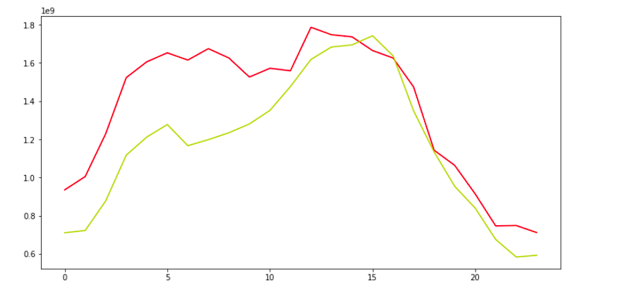
The forecasted values are almost close to the actual values. Well, the performance seems pretty much similar to that of the LSTM in the based model.
If You can recall in the Auto-tagging system project we saw that the CNN-based model outperform the LSTM based model by a huge margin.
But here in this case both the models have performed mode or less the same.
Conclusion
However, the CNN-based model still has the advantage of speed. Now, this is not the end of the row. We can further improve this model by taking measures like, we can make the time series data stationary and then use it for making sequences and then later use it in the model input sequences. To learn more about stationarity charity and other time series-related concepts, you can check out this link.
Apart from that, we can also try a different number of hidden units r different numbers of hidden layers. To see how our model performs under different settings. In addition, we can also try to change the learning rate. Even that might help in improving the model.
Author
Hi, I am Kajal Kumari. I have completed my Master’s from IIT(ISM) Dhanbad in Computer Science & Engineering. As of now, I am working as Machine Learning Engineer in Hyderabad. You can also check out few other blogs that I have written here.


