Introduction
Camera calibration is a fundamental task in computer vision crucial in various applications such as 3D reconstruction, object tracking, augmented reality, and image analysis. Accurate calibration ensures precise measurements and reliable analysis by correcting distortions and estimating intrinsic and extrinsic camera parameters. This comprehensive guide delves into the principles, techniques, and algorithms of camera calibration. We explore obtaining intrinsic and extrinsic camera parameters, understanding distortion models, conducting calibration patterns, and utilizing calibration software. Whether you are a beginner or an experienced computer vision practitioner, this guide will equip you with the knowledge and skills to perform accurate camera calibration matrix and unlock the full potential of your vision-based applications.
This article was published as a part of the Data Science Blogathon
Table of contents
- What is Camera Calibration?
- Types of Camera Calibration
- Camera Calibration Method
- Camera Calibration Models
- Types of distortion effects and their cause
- Mathematically Representing Lens Distortion
- Removing Distortion
- Python Code for Camera Calibration
- C++ Code for Camera Calibration
- Frequently Asked Questions
What is Camera Calibration?
A camera is a device that converts the 3D world into a 2D image. A camera plays a very important role in capturing three-dimensional images and storing them in two-dimensional images. To know the mathematics behind it is extremely fascinating. The following equation can represent the camera.
x=PX
Here x denotes 2-D image point, P denotes camera matrix and X denotes 3-D world point.
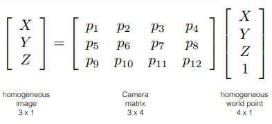
Figure1 vector representation of x=PX [1]
The image processing or computer vision field frequently uses the term “camera calibration.” The camera calibration method aims to identify the geometric characteristics of the image creation process. This vital step is necessary in many computer vision applications, especially when you need metric information on the scene. In these applications, you often classify the camera based on intrinsic parameters such as the skew of the axis, focal length, and principal point, while you describe its orientation with extrinsic parameters like rotation and translation. Linear or nonlinear algorithms estimate intrinsic and extrinsic parameters by utilizing known points in real-time and their projections in the picture plane.
Types of Camera Calibration
Camera calibration is the process of determining specific camera parameters in order to complete operations with specified performance measurements.
We can define camera calibration matrix as the technique used to estimate the characteristics of a camera. This involves obtaining all the necessary information such as parameters or coefficients of the camera to establish an accurate relationship between a 3D point in the real world and its corresponding 2D projection in the image captured by the calibrated camera.
In most cases, this entails recovering two types of parameters.
1. Intrinsic or Internal Parameters
It allows mapping between pixel coordinates and camera coordinates in the image frame. E.g. optical center, focal length, and radial distortion coefficients of the lens.
2. Extrinsic or External Parameters
It describes the orientation and location of the camera. This refers to the rotation and translation of the camera with respect to some world coordinate system.
Camera Calibration Method
This section will outline a simple calibration procedure. The key focus is on determining the correct focal length, as you can configure most parameters using basic assumptions such as square straight pixels and an optical center positioned in the middle of the image. To carry out this calibration method, you need a flat rectangular calibration object (such as a book), a measuring tape or ruler, and a flat surface. You can follow the steps below to conduct camera calibration matrix.
- Take a measurement of the length and width of your rectangle calibration object. Let us refer to these as dX and dY.
- Place the camera and calibration object on a flat surface with the camera back and calibration object parallel and the object roughly in the center of the camera’s vision. To acquire a good alignment, you may need to lift the camera or object.
- Calculate the distance between the camera and the calibration object. Let’s call it dZ.
- Take a picture to ensure that the setup is straight, which means that the sides of the calibration object align with the image’s rows and columns.
- In pixels, determine the width and height of the object. Let us refer to these as dx and dy.
Focal Length

Now let us see the following Figure-3 for set up.
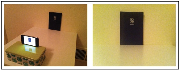
For the exact setup in Figure 4-3, the object was measured to be 130 by 185 mm, hence dX = 130 and dY = 185. The camera’s distance from the object was 460 mm, hence dZ = 460. Only the ratios of the measurements matter; any unit of measurement can be utilized. After using ginput() to choose four points in the image, the width and height in pixels were 722 and 1040, respectively. In other words, dx = 722 and dy = 1040. When these numbers are used in the aforementioned relationship, the result is
fx equals 2555, and fy equals 2586.
It is critical to note that this is only applicable to a specific image resolution. In this situation, the image was 2592 1936 pixels in size. It should be noted that focal length and optical center are mainly measured in pixels and scale with image resolution. If you choose a different image resolution, the values will change (for example, a thumbnail image). It’s a good idea to add your camera’s variables to a helper function like this:
def my_calibration(sz):
  row,col = sz
  fx = 2555*col/2592
  fy = 2586*row/1936
  K = diag([fx,fy,1])
  K[0,2] = 0.5*col
  K[1,2] = 0.5*row
  return K
After that, this function takes a size tuple and returns the calibration matrix. The optical center is assumed to be the image’s center in this case. Replace the focal lengths with their mean if you like; for most consumer cameras, this is fine. It should be noted that the calibration is only for photographs in landscape orientation.
Camera Calibration Models
Calibration techniques for the pinhole camera model and the fisheye camera model are included in the Computer Vision ToolboxTM. The fisheye variant is compatible with cameras with a field of vision (FOV) of up to 195 degrees.
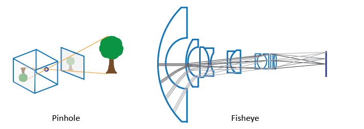
The pinhole calibration algorithm is based on Jean-Yves Bouguet’s [3] model. The pinhole camera model and lens distortion are included in the model. Because an ideal pinhole camera does not have a lens, the pinhole camera model does not account for lens distortion. To accurately simulate a genuine camera, the algorithm’s whole camera model incorporates radial and tangential lens distortion.
The pinhole model cannot model a fisheye camera due to the high distortion produced by a fisheye lens.
Pinhole Camera Model
A pinhole camera is a basic camera model without a lens. Light rays pass through the aperture and project an inverted image on the opposite side of the camera. Visualize the virtual image plane in front of the camera and assume that it is containing the upright image of the scene.
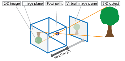
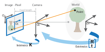
The camera matrix is a 4-by-3 matrix that represents the pinhole camera specifications. The image plane is mapped into the image plane by this matrix, which maps the 3-D world scene. Using the extrinsic and intrinsic parameters, the calibration algorithm computes the camera matrix. The extrinsic parameters represent the camera’s position in the 3-D scene. The intrinsic characteristics represent the camera’s optical center and focal length.
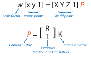
The extrinsic parameters transform the world points to camera coordinates, while the intrinsic parameters map the camera coordinates to the image plane.
Fisheye Camera Model
Camera Calibration Computer Vision is the process of calculating the extrinsic and intrinsic properties of a camera. After calibrating a camera, one can utilize the picture information to extract 3-D information from 2-D photographs. Images taken with a fisheye camera can also be distortion-free. In Matlab, there is the Computer Vision Toolbox which includes calibration procedures for the pinhole camera model and the fisheye camera model. The fisheye variation works with cameras that have a field of view (FOV) of up to 195 degrees.

As a fisheye lens produces extreme distortion, the pinhole model cannot model a fisheye camera.
Optically, fisheye cameras help solve simultaneous localization and mapping (SLAM) difficulties in addition to aiding in odometry. Surveillance systems, GoPro, virtual reality (VR) to capture a 360-degree field of view (fov), and stitching algorithms are examples of other applications. These cameras employ a complicated array of lenses to increase the camera’s field of view, allowing it to capture wide panoramic or hemispherical images. The lenses achieve this extraordinarily wide-angle view, however, by distorting the perspective lines
in the image.
The Computer Vision Toolbox calibration algorithm utilizes Scaramuzza’s fisheye camera model, which employs an omnidirectional camera model. The procedure treats the imaging system as a unified entity. To establish a connection between a 3-D world point and a 2-D image, you need to gather the camera’s extrinsic and intrinsic parameters. The extrinsic parameters map world points to camera coordinates, while the intrinsic parameters project the camera coordinates onto the picture plane.

Types of distortion effects and their cause
We obtain better photos when we use a lens, yet the lens produces some distortion effects. Distortion effects are classified into two types:
Radial Distortion
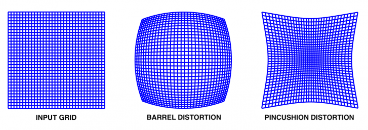
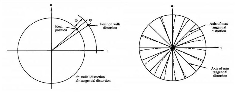
This sort of distortion is caused by unequal light bending. The rays bend more at the lens’s borders than they do at the lens’s center. Straight lines in the actual world appear curved in the image due to radial distortion. The light ray shifts radially inward or outward from its optimal point before hitting the image sensor. The radial distortion effect is classified into two types.
- Effect of barrel distortion, which corresponds to negative radial displacement
- The pincushion distortion effect results in a positive radial displacement.
Tangential Distortion
It occurs when the picture screen or sensor is at an angle with respect to the lens. As a result, the image appears to be slanted and stretched.
There are three types of distortion depending on the source: radial distortion, decentering distortion, and thin prism distortion. Decentering and narrow prism distortion both cause radial and tangential distortion.
We now have a better understanding of the different sorts of distortion effects generated by lenses, but what does a distorted image look like? Is it necessary to be concerned about the lens’s distortion? If so, why? How are we going to deal with it?
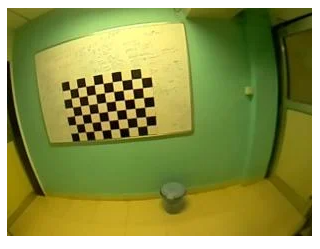
The image above is an example of the distortion effect that a lens can produce. The figure corresponds to figure 1 and is a barrel distortion effect, which is a form of the radial distortion effect. Which two points would you consider if you were asked to find the correct door height? Things get considerably more challenging when executing SLAM or developing an augmented reality application using cameras that have a large distortion effect in the image.
Mathematically Representing Lens Distortion
When attempting to estimate the 3D points of the real world from an image, we must account for distortion effects.
Based on the lens parameters, we mathematically analyze the distortion effect and combine it with the pinhole camera model described in the previous piece in this series. As additional intrinsic parameters, we have distortion coefficients (which quantitatively indicate lens distortion), in addition to the intrinsic and extrinsic characteristics discussed in the preceding post.
To account for these distortions in our camera model, we make the following changes to the pinhole camera model:
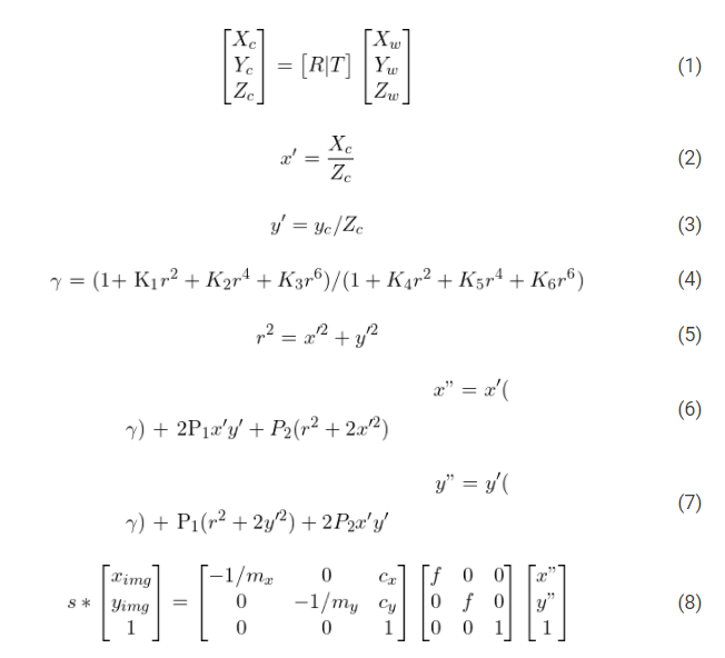
The calibrateCamera method returns the distCoeffs matrix, which contains values for K1 through K6, which represent radial distortion, and P1 and P2, which represent tangential distortion. Because the following mathematical model of lens distortion covers all sorts of distortions, radial distortion, decentering distortion, and thin prism distortion, the coefficients K1 through K6 represent net radial distortion while P1 and P2 represent net tangential distortion.
Removing Distortion
So what do we do after the calibration step? We got the camera matrix and distortion coefficients in the previous post on camera calibration computer vision but how do we use the values?
One application is to use the derived distortion coefficients to un-distort the image.The images shown below depict how lens distortion affects them and how you can remove it using the coefficients obtained from camera calibration computer vision.
How to Reduce Lens Distortion?
To reduce lens distortion, one must take three fundamental actions.
- Calibrate the camera and obtain the intrinsic camera parameters. This is exactly what we accomplished in the previous installment of this series. The camera distortion characteristics are also included in the intrinsic parameters.
- Control the percentage of undesired pixels in the undistorted image by fine-tuning the camera matrix.
- Using the revised camera matrix to remove distortion from the image.
The getOptimalNewCameraMatrix() method is used in the second phase. What exactly does this refined matrix imply, and why do we require it? Refer to the photographs below; in the right image, we can see several black pixels at the boundaries. These are caused by the image’s undistortion. These dark pixels are sometimes undesirable in the final undistorted image. Therefore, the getOptimalNewCameraMatrix() method provides a refined camera matrix along with the ROI (region of interest) that you can utilize to crop the image and eliminate all black pixels. The alpha parameter, which you input into the getOptimalNewCameraMatrix() method, determines the percentage of undesirable pixels to be removed.
Python Code for Camera Calibration
import cv2
 import numpy as np
 import os
 import glob
 # Defining the dimensions of checkerboard
 CHECKERBOARD = (6,9)
 criteria = (cv2.TERM_CRITERIA_EPS + cv2.TERM_CRITERIA_MAX_ITER, 30, 0.001)
 # Creating vector to store vectors of 3D points for each checkerboard image
 objpoints = []
 # Creating vector to store vectors of 2D points for each checkerboard image
 imgpoints = []
 # Defining the world coordinates for 3D points
 objp = np.zeros((1, CHECKERBOARD[0] * CHECKERBOARD[1], 3), np.float32)
 objp[0,:,:2] = np.mgrid[0:CHECKERBOARD[0], 0:CHECKERBOARD[1]].T.reshape(-1, 2)
 prev_img_shape = None
 # Extracting path of individual image stored in a given directory
 images = glob.glob('./images/*.jpg')
 for fname in images:
 img = cv2.imread(fname)
 gray = cv2.cvtColor(img,cv2.COLOR_BGR2GRAY)
 # Find the chess board corners
 # If desired number of corners are found in the image then ret = true
 ret, corners = cv2.findChessboardCorners(gray, CHECKERBOARD,
 cv2.CALIB_CB_ADAPTIVE_THRESH + cv2.CALIB_CB_FAST_CHECK + cv2.CALIB_CB_NORMALIZE_IMAGE)
 """
 If desired number of corner are detected,
 we refine the pixel coordinates and display
 them on the images of checker board
 """
 if ret == True:
 objpoints.append(objp)
 # refining pixel coordinates for given 2d points.
 corners2 = cv2.cornerSubPix(gray, corners, (11,11),(-1,-1), criteria)
 imgpoints.append(corners2)
 # Draw and display the corners
 img = cv2.drawChessboardCorners(img, CHECKERBOARD, corners2, ret)
 cv2.imshow('img',img)
 cv2.waitKey(0)
 cv2.destroyAllWindows()
 h,w = img.shape[:2]
 """
 Performing camera calibration by
 passing the value of known 3D points (objpoints)
 and corresponding pixel coordinates of the
 detected corners (imgpoints)
 """
 ret, mtx, dist, rvecs, tvecs = cv2.calibrateCamera(objpoints, imgpoints, gray.shape[::-1], None, None)
 print("Camera matrix : n")
 print(mtx)
 print("dist : n")
 print(dist)
 print("rvecs : n")
 print(rvecs)
 print("tvecs : n")
 print(tvecs)
C++ Code for Camera Calibration
#include
 #include
 #include
 #include
 #include
 #include
 // Defining the dimensions of checkerboard
 int CHECKERBOARD[2]{6,9};
 int main()
 {
   // Creating vector to store vectors of 3D points for each checkerboard image
   std::vector<std::vector > objpoints;
   // Creating vector to store vectors of 2D points for each checkerboard image
   std::vector<std::vector > imgpoints;
   // Defining the world coordinates for 3D points
   std::vector objp;
   for(int i{0}; i<CHECKERBOARD[1]; i++)
   {
     for(int j{0}; j<CHECKERBOARD[0]; j++)
       objp.push_back(cv::Point3f(j,i,0));
   }
// Extracting path of individual image stored in a given directory
   std::vector images;
   // Path of the folder containing checkerboard images
   std::string path = "./images/*.jpg";
   cv::glob(path, images);
   cv::Mat frame, gray;
   // vector to store the pixel coordinates of detected checker board corners
   std::vector corner_pts;
   bool success;
   // Looping over all the images in the directory
   for(int i{0}; i<images.size(); i++)
   {
     frame = cv::imread(images[i]);
     cv::cvtColor(frame,gray,cv::COLOR_BGR2GRAY);
     // Finding checker board corners
     // If desired number of corners are found in the image then success = true
     success = cv::findChessboardCorners(gray, cv::Size(CHECKERBOARD[0],
 CHECKERBOARD[1]), corner_pts, CV_CALIB_CB_ADAPTIVE_THRESH | CV_CALIB_CB_FAST_CHECK | CV_CALIB_CB_NORMALIZE_IMAGE);
     /*
      * If desired number of corner are detected,
      * we refine the pixel coordinates and display
      * them on the images of checker board
     */
     if(success)
     {
       cv::TermCriteria criteria(CV_TERMCRIT_EPS | CV_TERMCRIT_ITER, 30, 0.001);
       // refining pixel coordinates for given 2d points.
       cv::cornerSubPix(gray,corner_pts,cv::Size(11,11), cv::Size(-1,-1),criteria);
       // Displaying the detected corner points on the checker board
       cv::drawChessboardCorners(frame, cv::Size(CHECKERBOARD[0], CHECKERBOARD[1]), corner_pts, success);
       objpoints.push_back(objp);
       imgpoints.push_back(corner_pts);
     }
     cv::imshow("Image",frame);
     cv::waitKey(0);
   }
   cv::destroyAllWindows();
   cv::Mat cameraMatrix,distCoeffs,R,T;
   /*
    * Performing camera calibration by
    * passing the value of known 3D points (objpoints)
    * and corresponding pixel coordinates of the
    * detected corners (imgpoints)
   */
   cv::calibrateCamera(objpoints, imgpoints, cv::Size(gray.rows,gray.cols), cameraMatrix, distCoeffs, R, T);
   std::cout << "cameraMatrix : " << cameraMatrix << std::endl;
   std::cout << "distCoeffs : " << distCoeffs << std::endl;
   std::cout << "Rotation vector : " << R << std::endl;
   std::cout << "Translation vector : " << T << std::endl;
   return 0;
 }
Conclusion
Camera calibration is vital to computer vision, ensuring accurate measurements and reliable analysis in various applications. To enhance your understanding and proficiency in camera calibration, consider joining our Blackbelt program for Data Science. This comprehensive program equips learners with in-depth knowledge, hands-on experience, and industry-relevant skills to excel in computer vision and data science. Take advantage of the opportunity to become a proficient practitioner through the Blackbelt program and advance your career.
Reference
- http://www.cs.cmu.edu/~16385/s17/Slides/11.1_Camera_matrix.pdf
- https://www.sciencedirect.com/topics/computer-science/camera-calibration
- https://learnopencv.com/understanding-lens-distortion
- https://in.mathworks.com/help/vision/ug/camera-calibration.html
Frequently Asked Questions
A. Camera calibration is the process of estimating a camera’s intrinsic and extrinsic parameters to correct distortions and ensure accurate measurements in computer vision tasks. It involves determining factors such as focal length, principal point, and lens distortion coefficients.
A. Typically, one performs camera calibration by capturing images of a calibration pattern with known dimensions. These images extract feature points and match them to corresponding 3D world points. Solving the calibration equations allows us to estimate the camera parameters.
A. The function of camera calibration is to remove distortions caused by camera lenses and accurately relate image coordinates to real-world measurements. It enables precise measurements, object recognition, and accurate mapping in computer vision applications.
A. In OpenCV, camera calibration refers to estimating camera parameters using the functions and algorithms provided by the OpenCV library. OpenCV offers a comprehensive set of functions for camera calibration, including capturing images, finding calibration patterns, and calculating camera matrices and distortion coefficients.
The media shown in this article is not owned by Analytics Vidhya and are used at the Author’s discretion.


