Introduction
Imagine solving complex puzzles by learning from the coordinated movements of birds and fish. Particle Swarm Optimization (PSO) does just that. PSO Algorithm is an intelligent way of solving tricky problems by mimicking how creatures work together. PSO uses many tiny agents that move around to find the best answer. Each agent remembers its own best solution and the best solution from its neighbors. This helps them work together and find the best answer faster. As we explore PSO, we’ll uncover how this teamwork between virtual agents helps us crack challenging problems in different areas.
Table of contents
- What is PSO Algorithm?
- Group optimization and Ensemble Learning
- The Problem of Optimization
- Mathematical Formulation of an Optimization Problem
- An Intuition of PSO Algorithm
- Particle Swarm Optimization Algorithm
- Analysis of the Particle Swarm Optimization Algorithm
- Neighborhood Topologies
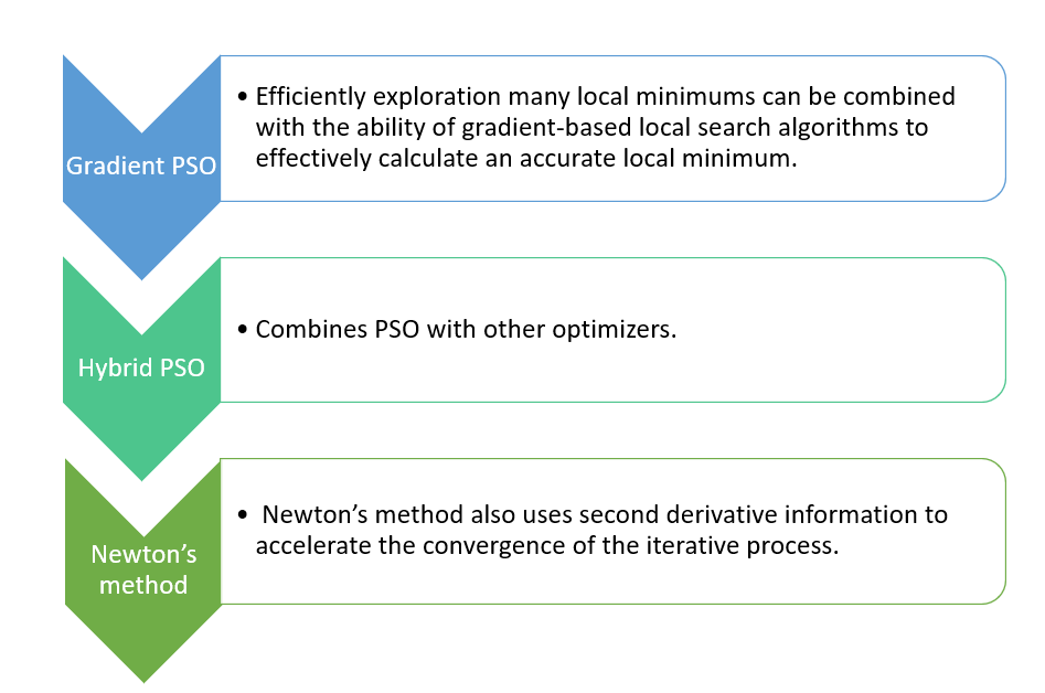
- Types of Particle Swarm Optimization
- Contour Plot
- Difference between PSO and Genetic Algorithm
- Advantages and disadvantages of Particle Swarm Optimization
- Conclusion
- Frequently Asked Question
What is PSO Algorithm?
The Particle Swarm Optimization (PSO) algorithm is a computational technique inspired by the collective behavior of natural organisms, such as birds or fish, that move together to achieve a common goal. In PSO, a group of particles (representing potential solutions) navigates through a problem’s solution space to find the best possible solution. Each particle adjusts its position based on its own best-known solution (personal best) and the best solution discovered by the entire group (global best). This collaborative movement enables particles to converge toward optimal solutions over iterations. PSO is widely used for optimization problems in various fields, leveraging the power of collective intelligence to explore complex solution spaces and find optimal outcomes efficiently.

Group optimization and Ensemble Learning
Many of you might have encountered the concept of ‘No Free Lunch (NFL)’ in machine learning. It suggests that no single model is universally superior for all scenarios. In simpler terms, different optimization algorithms can perform equally well when averaged across various problems. To illustrate this idea, consider a flock of birds. Now, why do optimization techniques matter in machine learning and deep learning? When training a model, we define a loss function that quantifies the difference between our model’s predictions and actual values. The aim is to minimize or optimize this loss function, driving it closer to zero.
Understanding Ensemble Learning
You might have also encountered the term ‘Ensemble Learning.’ If not, let me clarify. ‘Ensemble’ is derived from the French word meaning ‘Assembly.’ It revolves around learning in a collective or group manner. Imagine training a model using multiple algorithms. What advantages does this offer? A single-base learner is considered weak. However, when these individual learners unite, they become stronger. This amalgamation enhances their predictive power, accuracy, and precision while reducing error rates. This combined model is called ‘Meta-learning’ in machine learning, where algorithms learn from other algorithms. This approach minimizes variance, bias, and enhances predictive capabilities. Achieving this level of proficiency can be likened to an ultimate ‘Nirvana’ moment for a data analyst.
Checkout our Comprehensive Guide to Ensemble Learning (with Python codes).
The Problem of Optimization
Now let’s come back to our PSO model. The concept of swarm intelligence inspired the POS. Here we are speaking about finding the optimal solution in a high-dimensional solution space. It talks about Maximizing earns or minimizing losses. So, we are looking to maximize or minimize a function to find the optimum solution. A function can have multiple local maximum and minimum. But, there can be only one global maximum as well as a minimum. If your function is very complex, then finding the global maximum can be a very daunting task. PSO tries to capture the global maximum or minimum. Even though it cannot capture the exact global maximum/minimum, it goes very close to it. It is the reason we called PSO a heuristic model.
Finding of Global Maximum or Minimum
Let me give you an example of why the finding of global maximum/minimum is problematic. Check the below function :
y=f(x)=sinx+sinx2+sinxcosx
If we plot this function, it looks like below:
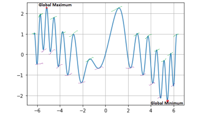
We can see that we have one global maximum and one global minimum. If we consider the function based on an interval in X-axis value from -4 to 6, we will have a maximum that will not be our global maximum. It is a local maximum. So we can say that finding out the global maximum may depend upon the interval. It is something like we try to observe a portion of a continuous function. Also, one thing to note while describing a dynamic system or entity, you can not have a static function. The function that I have defined here is fixed. Data analytics is data-hungry. To train a model or to find a suitable mathematical function, you must have enormous data.
It is impossible to have all the data. Meaning it’s challenging to get the exact global minimum or maximum. Well, for me, it’s a limitation of Mathematics. Fortunately, we have Statistics that advocate sampling, and from there, it can optimize some value like global maximum or minimum concerning the original function. But again, you won’t get the exact global maximum or minimum. You will get some values that will be closer to the actual global maximum or minimum.
PSO Example with Multiple Variables
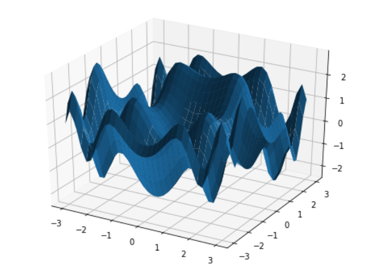
Also, when we describe a mathematical function based on some real-life scenario, we must explain it with multiple variables or higher-dimensional vector space. The growth of bacteria in a jar may depend upon temperature, humidity, the container, the solvent, etc. For this type of function, it’s more challenging to get the exact global maximum and minimum. Check the below function. And see if we add more variables than how difficult it becomes to get global maximum and minimum.
z=f(x, y)=sin x2+siny2+sinxsiny
Mathematical Formulation of an Optimization Problem
In the optimization problem, we have a variable represented by a vector X=[x1x2x3…xn] that minimizes or maximizes cost function depending on the proposed optimization formulation of the function f(X). X is known as position vector; it represents a variable model. It is an n dimensions vector, where n represents the number of variables determined in a problem. We can call it latitude and the longitude in the problem of choosing a point to land by a flock of birds. The function f(X) is called the fitness function or objective function. The job of f(X) is to assess how good or bad a position X is; that is, how perfect a certain landing point a bird thinks after finding a suitable place. Here, the evaluation, in this case, is performed through several survival criteria.
An Intuition of PSO Algorithm
The movement towards a promising area to get the global optimum.
- Each particle adjusts its traveling velocity dynamically, according to the flying experiences it has and its colleagues in the group.
- Each particle tries to keep track of :
- It’s best result for him/her, known as personal best or pbest.
- The best value of any particle is the global best or gbest.
- Each particle modifies its position according to:
- Its current position
- Its current velocity
- The distance between its current position and pbest.
- The distance between its current position and gbest.
Particle Swarm Optimization Algorithm
Lets us assume a few parameters first. You will find some new parameters, which I will describe later.
- f: Objective function
- Vi: Velocity of the particle or agent
- A: Population of agents
- W: Inertia weight
- C1: cognitive constant
- U1, U2: random numbers
- C2: social constant
- Xi: Position of the particle or agent
- Pb: Personal Best
- gb: global Best
The actual algorithm goes as below :
1. Create a ‘population’ of agents (particles) which is uniformly distributed over X.
2. Evaluate each particle’s position considering the objective function( say the below function).
z=f(x, y)=sin x2+siny2+sinxsiny
3. If a particle’s present position is better than its previous best position, update it.
4. Find the best particle (according to the particle’s last best places).
5. Update particles’ velocities.

6. Move particles to their new positions.

7. Go to step 2 until the stopping criteria are satisfied.
Analysis of the Particle Swarm Optimization Algorithm
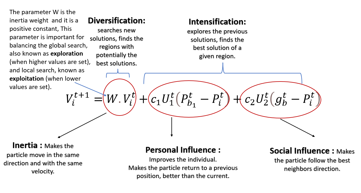
If W=1, the particle’s motion is entirely influenced by the previous motion, so the particle may keep going in the same direction. On the other hand, if 0≤W<1, such influence is reduced, which means that a particle instead goes to other regions in the search domain.
Pb1t And its current position Pit. It has been noticed that the idea behind this term is that as the particle gets more distant from the Pb1t (Personal Best) position, the difference (Pb1t-Pit ) Must increase; hence, this term increases, attracting the particle to its best own position. The parameter C1 existing as a product is a positive constant, and it is an individual-cognition parameter. It weighs the importance of the particle’s own previous experiences.
The other hyper-parameter which composes the product of the second term is U1t. It is a random value parameter with [0,1] range. This random parameter plays an essential role in avoiding premature convergences, increasing the most likely global optima.
The difference (gbt-Pit ) Works as an attraction for the particles towards the best point until it’s found at t iteration. Likewise, C2 is also a social learning parameter, and it weighs the importance of the global learning of the swarm. And U2t plays precisely the same role as U1t.
- C1=C2=0, all particles continue flying at their current speed until they hit the search space’s boundary.
- C1>0 and C2=0, all particles are independent.
- C1>0 and C2=0, all particles are attracted to a single point in the entire swarm.
- C1=C2≠0, all particles are attracted towards the average of pbest and gbest.
Neighborhood Topologies
A neighborhood must be defined for each particle. This neighborhood determines the extent of social interaction within the swarm and influences a particular particle’s movement. Less interaction occurs when the neighborhoods in the swarm are small. For small neighborhoods, the convergence will be slower, but it may improve the quality of solutions. The convergence will be faster for more prominent neighborhoods, but the risk that sometimes convergence occurs earlier.
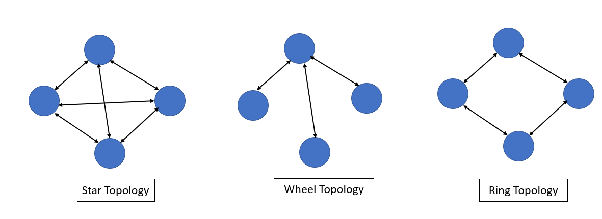
For Star topology, each particle is connected with other particles. It leads to faster convergence than other topologies, Easy to find out gbest. But it can be biased to the pbest.
For wheel topology, only one particle connects to the others, and all information is communicated through this particle. This focal particle compares the best performance of all particles in the swarm, and adjusts its position towards the best performance particle. Then the new position of the focal particle is informed to all the particles.
For Ring Topology, when one particle finds the best result, it will make pass it to its immediate neighbors, and these two immediate neighbors pass it to their immediate neighbors until it reaches the last particle. Here the best result found is spread very slowly.
Types of Particle Swarm Optimization
Contour Plot
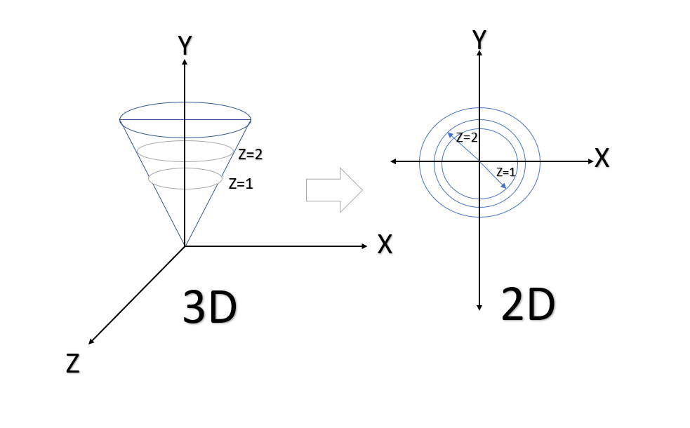
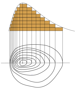
It is a graphical technique to represent 3 -Dimensional surface in 2- dimensional Plot using variable Z in the form of slices known as contours. I hope the below example can give you the intuition.
Let’s draw a graph of circle z=x2+y2 at fixed heights ‘z’ , z =1,2,3 etc.
To give you intuition, let Plot the function below in the contour plot.
z=x2+y2 its actual plotting and the contour plotting will look like below:
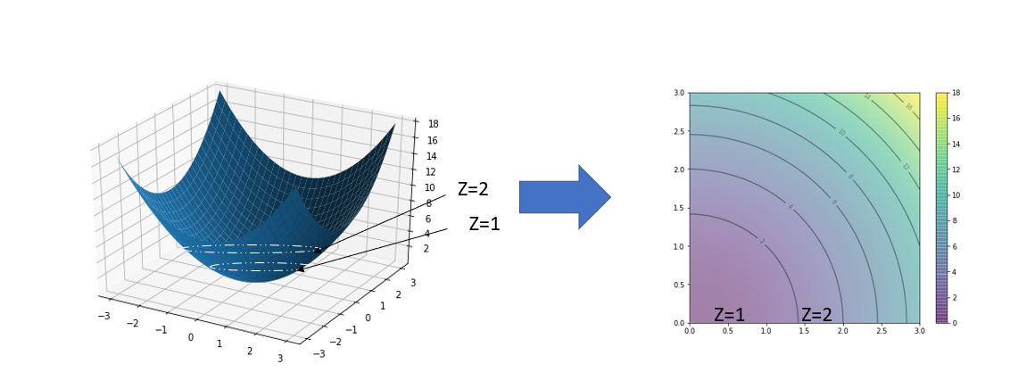
Here we can see the function in the region of f(x,y). We can create ten particles at random locations in this region, together with a random velocity which is sampled over a normal distribution with mean 0 and standard deviation 0.1, as follows:
.png)
The actual outcome will be like :
PSO found best solution at f([0.01415657 0.65909248])=0.4346033028251361
Global optimal at f([0.0, 0.0])=0.0
For details coding part, I’ll highly recommend you to visit the link: https://machinelearningmastery.com/a-gentle-introduction-to-particle-swarm-optimization/
Also, there is a library available called as pyswarms; please check here to know more!
Difference between PSO and Genetic Algorithm
Genetic Algorithms (GAs) and PSOs are both used as cost functions, they are both iterative, and they both have a random element. They can be used on similar kinds of problems. The difference between PSO and Genetic Algorithms (GAs) is that GAs it does not traverse the search space like birds flocking, covering the spaces in between. The operation of GAs is more like Monte Carlo, where the candidate solutions are randomized, and the best solutions are picked to compete with a new set of randomized solutions. Also, PSO algorithms require normalization of the input vectors to reach faster “convergence” (as heuristic algorithms, both don’t truly converge). GAs can work with features that are continuous or discrete.
Also, In PSO, there is no creation or deletion of individuals. Individuals merely move on a landscape where their fitness is measured over time. This is like a flock of birds or other creatures that communicate.
Advantages and disadvantages of Particle Swarm Optimization
Advantages :
- Insensitive to scaling of design variables.
- Easily parallelized for concurrent processing.
- Derivative free.
- Very few algorithm parameters.
- A very efficient global search algorithm.
Disadvantages :
- PSO’s optimum local searchability is weak
Conclusion
The most exciting part of PSO Algorithm is there is a stable topology where particles are able to communicate with each other and increase the learning rate to achieve global optimum. The metaheuristic nature of this optimization algorithm gives us lots of opportunities as it optimizes a problem by iteratively trying to improve a candidate solution. Applicability of it will increase more with the ongoing research work in Ensemble Learning.
Frequently Asked Question
A. Particle Swarm Optimization (PSO) simulates the social behavior of birds or fish, where particles (solutions) move through a solution space, adjusting their positions based on their own best-known solution and the collective knowledge of the swarm.
A. PSO is used to optimize complex problems by iteratively improving solutions based on particle movement and their interactions, making it effective for optimization tasks in various fields.
A. PSO was introduced by Dr. Eberhart and Dr. Kennedy in 1995, inspired by the social behaviors of birds and fish.
A. PSO finds applications in diverse fields, including engineering design, neural network training, economic modeling, data clustering, and parameter tuning in machine learning algorithms.
The media shown in this article is not owned by Analytics Vidhya and are used at the Author’s discretion.


Inequality functions c1 ,c2 kindly check c1 greater than 0 (two cases given) second one c2greater than 0?
You did a fantastic job. Thank you.