Perceptron: Building Block of Artificial Neural Network

If you are a machine learning and AI enthusiast, you must have come across the word perceptron. Perceptron is taught in the first chapter of many deep learning courses. So what exactly it is? What is the inspiration behind it? How exactly it solves the classification problem? In this article, we are going to start with the biological inspiration behind the perceptron and then delve into its mathematical technicalities, and finally build a binary classifier from scratch using a perceptron unit.

This article was published as a part of the Data Science Blogathon

What is Perceptron?

A perceptron is a basic unit in neural networks, mimicking brain neurons. It processes inputs with weighted connections and a bias, producing binary outputs through an activation function. Primarily used in binary classification tasks, perceptrons were instrumental in advancing neural network development and deep learning techniques.

What characterizes the Perceptron model in machine learning?

The Perceptron model in machine learning is characterized by the following key points:

• Binary Linear Classifier: The Perceptron is a type of binary classifier that assigns input data points to one of two possible categories.

• Input Processing: It takes multiple input signals and processes them, each multiplied by a corresponding weight. The inputs are aggregated, and the model produces a single output.

• Activation Function: The Perceptron uses an activation function, typically a step function, to determine the output based on the aggregated inputs and weights. If the result exceeds a certain threshold, the output is one category; otherwise, it’s the other.

• Training Process: During training, the model adjusts its weights based on the error in its predictions compared to the actual outcomes. This adjustment helps improve the model’s accuracy over time.

• Single-Layer Model: The Perceptron is a single-layer neural network since it has only one layer of output after processing the inputs.

• Limitations: While effective for linearly separable data, the Perceptron has limitations in handling more complex patterns, leading to the development of more sophisticated neural network architectures.

Understanding the Perceptron is crucial as it forms the foundation for more advanced neural network structures used in modern machine learning applications.

The Fundamentals of Neural Networks

Neural networks are a type of machine learning model inspired by the structure and function of the human brain. They are composed of interconnected nodes, called neurons, organized into layers. Each neuron receives input, processes it through an activation function, and produces an output. The connections between neurons are represented by weights, which are adjusted during the learning process to optimize the network’s performance.

The basic building block of a neural network is the perceptron, which consists of one or more input nodes, weights associated with each input, a summation function to combine the inputs and weights, and an activation function to produce the predicted output. Perceptrons can be stacked together to form more complex architectures, such as single-layer perceptrons or multi-layer perceptrons (MLPs).

Training a neural network involves feeding it a set of input-output pairs (training data) and adjusting the weights to minimize the difference between the network’s predictions and the actual outputs. This process, often referred to as supervised learning, utilizes techniques like gradient descent to iteratively update the weights based on the error between the predicted and actual outputs.

One of the challenges in training neural networks is handling linearly separable patterns within the input data computations. Techniques such as regularization, dropout, and cross-validation are employed to mitigate overfitting and enhance the network’s ability to generalize to unseen data.

Neural networks have shown remarkable success in various applications, including image and speech recognition, natural language processing, and reinforcement learning. Their ability to learn complex patterns and relationships from data, facilitated by artificial neurons, makes them a powerful tool in modern machine learning and artificial intelligence.

Biological inspiration of Neural Networks

A neuron (nerve cell) is the basic building block of the nervous system. A human brain consists of billions of neurons that are interconnected to each other. They are responsible for receiving and sending signals from the brain. As seen in the below diagram, a typical neuron consists of the three main parts – dendrites, an axon, and cell body or soma. Dendrites are tree-like branches originating from the cell body. They receive information from the other neurons. Soma is the core of a neuron. It is responsible for processing the information received from dendrites. Axon is like a cable through which the neurons send the information. Towards its end, the axon splits up into many branches that make connections with the other neurons through their dendrites. The connection between the axon and other neuron dendrites is called synapses.

Image Source: Willems, K. (2017, May 2). Keras Tutorial: Deep Learning in Python.

As ANN is inspired by the functioning of the brain, let us see how the brain works. The brain consists of a network of billions of neurons. They communicate by means of electrical and chemical signals through a synapse, in which, the information from one neuron is transmitted to other neurons. The transmission process involves an electrical impulse called ‘action potential’. For the information to be transmitted, the input signals (impulse) should be strong enough to cross a certain threshold barrier, then only a neuron activates and transmits the signal further (output).

Inspired by the biological functioning of a neuron, an American scientist Franck Rosenblatt came up with the concept of perceptron at Cornell Aeronautical Laboratory in 1957.

• A neuron receives information from other neurons in form of electrical impulses of varying strength.
• Neuron integrates all the impulses it receives from the other neurons.
• If the resulting summation is larger than a certain threshold value, the neuron ‘fires’, triggering an action potential that is transmitted to the other connected neurons.

Main Components of Perceptron

Rosenblatt’s perceptron is basically a binary classifier. The perceptron consists of 3 main parts:

• Input nodes or input layer: The input layer takes the initial data into the system for further processing. Each input node is associated with a numerical value. It can take any real value.
• Weights and bias: Weight parameters represent the strength of the connection between units. Higher is the weight, stronger is the influence of the associated input neuron to decide the output. Bias plays the same as the intercept in a linear equation.
• Activation function: The activation function determines whether the neuron will fire or not. At its simplest, the activation function is a step function, but based on the scenario, different activation functions can be used.

We shall see more about these in the subsequent section.

Working of a Perceptron

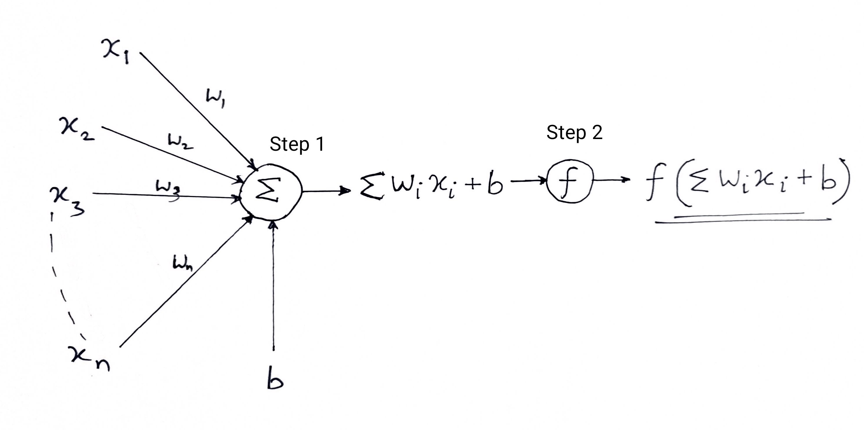
In the first step, all the input values are multiplied with their respective weights and added together. The result obtained is called weighted sum ∑wi*xi, or stated differently,  x1*w1 + x2*w2 +…wn*xn. This sum gives an appropriate representation of the inputs based on their importance. Additionally, a bias term b is added to this sum ∑wi*xi + b. Bias serves as another model parameter (in addition to weights) that can be tuned to improve the model’s performance.

In the second step, an activation function f is applied over the above sum ∑wi*xi + b to obtain output Y = f(∑wi*xi + b). Depending upon the scenario and the activation function used, the Output is either binary {1, 0} or a continuous value. 

(Often both these steps are represented as a single step in multi-layer perceptrons, here I have shown them as two different steps for better understanding)

Activation Functions

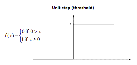
A biological neuron only fires when a certain threshold is exceeded. Similarly, the artificial neuron will also only fire when the sum of the inputs (weighted sum) exceeds a certain threshold value, let’s say 0. Intuitively, we can think of a rule-based approach like this –

If  ∑wi*xi + b > 0:
    output = 1
else:
    output = 0

Its graph will be something like this:

This is in fact the Unit Step (Threshold) activation function which was originally used by Rosenblatt. But as you can see, this function is discontinuous at 0, so it causes problems in mathematical computations. A smoother version of the above function is the sigmoid function. It outputs between 0 and 1. Another one is the Hyperbolic tangent(tanh) function, which produces the output between -1 and 1. Both sigmoid and tanh functions suffer from vanishing gradients problems. Nowadays, ReLU and Leaky ReLU are the most popularly used activation functions. They are comparatively stable over deep networks.

Perceptron as a Binary Classifier

So far, we have seen the biological inspiration and the mathematics of the perceptron. In this section, we shall see how a perceptron solves a linear classification problem.

Importing some libraries –

from sklearn.datasets import make_blobs
import matplotlib.pyplot as plt
import numpy as np
%matplotlib inline

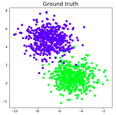
Generating a dummy dataset using make_blobs functionality provided by scikit learn –

# Generate dataset
X, Y = make_blobs(n_features = 2, centers = 2, n_samples = 1000, random_state = 12)
# Visualize dataset
plt.figure(figsize = (6, 6))
plt.scatter(X[:, 0], X[:, 1], c = Y)
plt.title('Ground truth', fontsize = 18)
plt.show()

Let’s say the blue dots are 1s and the green dots are 0s. Using perceptron logic, we can create a decision boundary(hyperplane) for classification which separates different data points on the graph.

Before we proceed further, let’s add a bias term (ones) to the input vector –

# Add a bias to the input vector
X_bias = np.ones([X.shape[0], 3])
X_bias[:, 1:3] = X

The dataset will look something like this – 

Here each row of the above dataset represents the input vector (a datapoint). In order to create a decision boundary, we need to find out the appropriate weights. The weights are  ‘learned’ from the training using the below rule –

w = w + (expected — predicted) * x

It means that subtracting the estimated outcome from the ground truth and then multiplying this by the current input vector and adding old weights to it in order to obtain the new value of the weights. If our output is the same as the actual class, then the weights do not change. But if our estimation is different from the ground truth, then the weights increase or decrease accordingly. This is how the weights are progressively adjusted in each iteration.

We start by assigning arbitrary values to the weight vector, then we progressively adjust them in each iteration using the error and data at hand –

# initialize weights with random values
w = np.random.rand(3, 1)
print(w)

Output:

[[0.37547448]
 [0.00239401]
 [0.18640939]]

Define the activation function of perceptron –

def activation_func(z):
    if z >= 1:
        return 1
    else:
        return 0
Next, we apply the perceptron learning rule -

for _ in range(100):
     for i in range(X_bias.shape[0]):
         y = activation_func(w.transpose().dot(X_bias[i, :]))
         # Update weights
         w = w + ((Y[i] - y) * X_bias[i, :]).reshape(w.shape[0], 1)

It is not guaranteed that the weights will converge in one pass, so we feed all the training data into the perceptron algorithm 100 times while constantly applying the learning rule so that eventually we manage to obtain the optimal weights.

Now, that we have obtained the optimal weights, we predict the class for each datapoint using Y = f(∑wi*xi + b) or Y = wT.x in vector form.

# predicting the class of the datapoints
result_class = [activation_func(w.transpose().dot(x)) for x in X_bias]

Visualize the decision boundary and the predicted class labels –

# convert to unit vector
w = w/np.sqrt(w.transpose().dot(w))
# Visualize results
plt.figure(figsize = (6, 6))
plt.scatter(X[:, 0], X[:, 1], c = result_class)
plt.plot([-10, -1], hyperplane([-10, -1], w), lw = 3, c = 'red')
plt.title('Perceptron classification with decision boundary')
plt.show()

You can compare the ground truth image with the predicted outcome image and see some points that are misclassified. If we calculate the accuracy, it comes to about 98% (I leave this as an exercise to the readers).

If you see, here our original data was fairly separated, so we are able to get such good accuracy. But this is not the case with real-world data. Using a single perceptron, we can only construct a linear decision boundary, so if the data is intermixed the perceptron algorithm will perform poorly. This is one of the limitations of the single perceptron model.

End Notes

We started by understanding the biological inspiration behind Rosenblatt’s perceptron. Then we progressed to the mathematics of perceptron and the activation functions. Finally using a toy dataset, we saw how perceptron can perform basic classification by building a linear decision boundary that separates the datapoints belonging to different classes.

Frequently Asked Questions