This article was published as a part of the Data Science Blogathon.
Introduction
In the field of Data Science, the most important thing is to prepare the data or clean the data for further model building, data exploration, or
data visualization, etc. For this Pandas is a very powerful library in python because it has a lot of inbuilt functions. In this article, I will cover a complete guide to a pandas data frame with a lot of examples and implementations i.e how to clean the data in the easiest way with fewer efforts.
In this article you will see the following:
- Installation
- How create the DataFrame?
- Read different types of files in a DataFrame
- Handle missing values
- Various operations on DataFrame
- Rename the features.
- GroupBy function
- Mathematical operations on the data
- Data visualization
Let’s start with the installation procedure of pandas in your system.
Installation of Pandas
The setup would take place in Google Colab Notebook. You can open Colab Notebook using the link.
Colab Notebooks are Jupyter Notebooks that run on the cloud. It is also connected with our google drive so which makes it easier to access our Colab notebooks from any place.
We can install pandas by using the pip command. Just type !pip install pandas in the cell and run the cell it will install the library.
!pip install pandas

After installation, you can check the version and import the library just to make sure if installation is done correctly or not.
import pandas as pd
print(pd.__version)
Create Pandas DataFrame
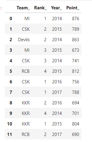
DataFrame is a structure that contains data in two-dimensional and corresponding to its labels. DataFrame is similar to SQL tables or excels sheets. In many cases, DataFrame is faster and easier to use, & powerful than spreadsheets or excel sheets/CSV files because they are an integral part of the python and NumPy library. To create a pandas DataFrame there are several ways but you will see the easiest way to create a pandas DataFrame in this article. we will create the DataFrame from dict of narray/list, where lengths of all the arrays will be the same.
import pandas as pd
points_table = {'Team_':['MI', 'CSK', 'Devils', 'MI', 'CSK',
   'RCB', 'CSK', 'CSK', 'KKR', 'KKR', 'KKR', 'RCB'],
   'Rank_' :[1, 2, 2, 3, 3,4 ,1 ,1,2 , 4,1,2],
   'Year_' :[2014,2015,2014,2015,2014,2015,2016,2017,2016,2014,2015,2017],
   'Point_':[876,789,863,673,741,812,756,788,694,701,804,690]}
df = pd.DataFrame(points_table)
pritn(df)
Instead of creating a data frame manually, If you want you can easily read the file in the
pandas DataFrame. You can read various types of files such as
txt, CSV, Excel, XML, SQL, etc.
pd.read_csv()
dataframe=pd.read_csv("file.csv")
This is the list of parameters it takes with its default values.
pandas.read_csv(filepath_or_buffer,
sep=NoDefault.no_default, delimiter=None, header='infer',
names=NoDefault.no_default, index_col=None, usecols=None, squeeze=False,
prefix=NoDefault.no_default, mangle_dupe_cols=True, dtype=None,
engine=None, converters=None, true_values=None, false_values=None,
skipinitialspace=False, skiprows=None, skipfooter=0, nrows=None,
na_values=None, keep_default_na=True, na_filter=True, verbose=False,
skip_blank_lines=True, parse_dates=False, infer_datetime_format=False,
keep_date_col=False, date_parser=None, dayfirst=False, cache_dates=True,
iterator=False, chunksize=None, compression='infer', thousands=None,
decimal='.', lineterminator=None, quotechar='"', quoting=0,
doublequote=True, escapechar=None, comment=None, encoding=None,
encoding_errors='strict', dialect=None, error_bad_lines=None,
warn_bad_lines=None, on_bad_lines=None, delim_whitespace=False,
low_memory=True, memory_map=False, float_precision=None,
storage_options=None)
Not all of them are important but remembering these will save you a lot of time while doing data cleaning. Some of the frequently used parameters are:
file_path: location of the file.
sep: It stands for the separator, its default value is ‘,’ in CSV file.
names: List of column names to use.
index_col: It is used to set the index columns instead of 0,1,2,3… which is default value
nrows: Number of rows to read from the large files.
na_filter: bool, default True It will help to detect the missing value of loading the data without NA value if it is set to false.
Sometimes Pandas DataFrames are very large that it is impossible to see all the data at the same time. So for this, there are several methods to access the data. The head(n) method is used to show first n rows (n is optional its default value is 5) if you want to see the last n rows you can use the tail() function similarly if you want to see n random rows from the dataset then we can use sample() function. In this article, we will be using the diabetes.csv dataset.
Head:
df=pd.read_csv("../input/pima-indians-diabetes-database/diabetes.csv")
#this will give first 5 rows of the data frame we can also get the first 10 the rows n=10
df.head(n=5)

Tail:
#this will give last5 rows of the dataframe we can also get the last 10 the rows n=10
df.tail(n=5)

Sample:
#this will give random 5 rows of the dataframe we can also get the random 10 the rows n=10
df.sample()

Columns:
#this will the all the name of attributes in the dataframre
df.columns

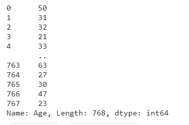
In pandas DataFrame, you can easily access the specific column or row. For accessing the specific columns you can specify the column name in “[]” brackets.
Access records:
age=df['Age']
print(age)
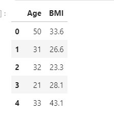
if you want to select multiple columns then you need to pass the array/list of the feature names.
df[['Age','BMI']].head()
For accessing the number of rows we can get it just like we get it from the python list.
df[0:4] 0 to 4 rows from the dataset

or you can use iloc() and loc() functions
iloc() is a indexed based on selection method that we have to pass index specific values of rows and columns, we can also pass the range of the index values now let’s check how you can do the same.
Loc:
df.loc[[2,4,6,7,8,9,19 ]] #it will select the 2th,4th,6th,7th,8th,9th,11th rows from the dataframe
df.loc[[2,5,9,15,16]]

ILoc:
df.iloc([ 2:8,2:5]) #this will select the rows from  2 to 8 and coluumns from 2 to 5 with the index values .
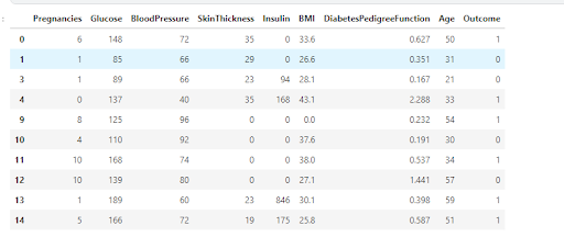
df.iloc[0:5,0:3]
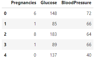
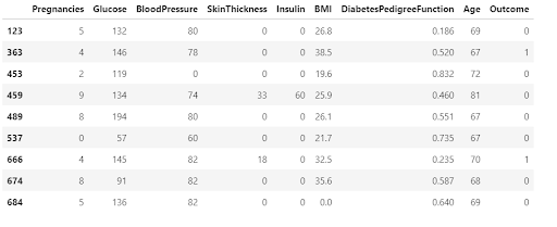
The loc() function is used to retrieve the group of rows and columns by labels or boolean array in the DaraFrame. It only takes index labels, and it exists in the data frame and returns all the rows, columns.
df.loc[df['Age']>66]
Rename:
In pandas, we have rename() function with the help of this we can rename the various features names or multiple features at the same time.
df.rename(columns={"Age": "age", "DiabetesPedigreeFunction": "DBF"}).head()

Drop:
We use the drop() function for deleting the specific column or to delete the multiple columns at the same time. The drop() function will take various parameters so let’s discuss all of them.
DataFrame.drop(labels=None, axis=0, index=None, columns=None, level=None, inplace=False, errors=’raise’)
labels: single label or list (index or name of the columns to drop).
axis: {0 or ‘index’, 1 or ‘columns’}, it’s default value is 0.
columns: It is the same as the label or we can say that it is an alternative to specify the names of the attributes (colums=labels).
level: If there are multiple indexes present in the DataFrame then we will pass the level.
inplace: If false then return a copy .otherwise do operation inplace and return none.
df.drop(  labels=['Age','BMI'],
axis=1,
inplace=True
)

If you want to drop the rows then we will simply pass the index values and set the axis =0 for the rows and in labels pass the index
value of the rows.
df.drop(
labels=[ 2,5,6,8,7],
axis=0,
inplace=True
)
This will drop the rows with index values 2, 4, 6, 8, 7.
Handle Missing Values using Pandas dataframe operations
In a DataFrame, the most important work is to handle the missing values or NA values because the presence of missing values does not enable Machine Learning models to learn that’s why we need to handle these very carefully. For handling the missing values we have various methods such as filling it with specific values such as zero, or we can fill it with the mean, median, or mode of the whole data and also there are more methods let’s check them out:
To understand it easily let’s create a DataFrame.
df = pd.DataFrame([[
    np.nan, 2, np.nan, 0],
     [3, 4, np.nan, 1],
     [np.nan, np.nan, np.nan, 5],
     [np.nan, 3, np.nan, 4]],
     columns=list("ABCD"))
print(df)
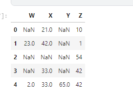
Let’s find the total number of NA values present on our DataFrame.
df.isna().sum()

Fill NA:
If you want to replace all the NA values with a specific number or especially with zero then you can use the fillna() function which will take various arguments.
DataFrame.fillna(value=None, method=None, axis=None, inplace=False, limit=None, downcast=None)
value: Specific value with which NA will be replaced.
method: {“backfill”,”bfill”,”pad”,”ffill”,None}, these all are the methods to fill the na values.
If you want to replace the NA values from the backward and forward values present in the data then you can use “bfill” and “ffill”.
axis: {0 or “index”,1 or”column”}, Axis along which to fill missing values.
limit: This is the maximum number of NA values to be filled with in the axis.
Let’s implement all of these methods:-
#Let's fill all the NA values with specific integer or zero
df.fillna(0)
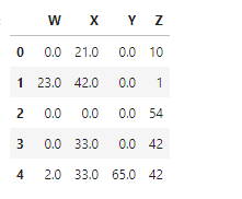
limit = 2 means only two NA values are filled with 0 or in a row if more than two NA values are present then only the first two Na values are
filled with zero if we will pass the limit=2.
df.fillna(0,limit=2)
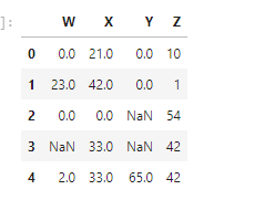
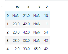
The ‘ffill’ is a forward fill in this method the values are filled with the values present in the next row. Similarly, you can use the “bfill” for the backward fill it will take the values which is present in the previous row.
df.fillna(method='ffill)
Source: Local
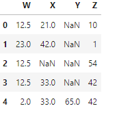
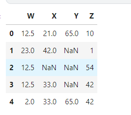
You can also fill the NA values with the mean, mode, or median.
df['W'].fillna(df['W'].mean() ,inplace=True)
Source: Local
df['W'].fillna(df['W'].mode() ,inplace=True)
Source: Local
Drop NA:
Or you can simply drop all the NA values by using the dropna() function.
Dataframe.dropna(labels=None,axis=0,how=”any”,thresh=None,subset=None,inplace=False)
axis: Determine if rows or columns will contain missing values. axis =0 or ‘index’ means drop the Na values within a row. axis=1 or ‘columns’ means to drop the Na values within the columns
how: {”any”,”all”} default ‘any’
subset: If you want to drop NA values from specific or multiple columns.
inplace: Replaces the output DataFrame with the current DataFrame.
This will drop all the rows if there is any NA value present.
df.dropna(inplace=True)

GroupBy Function
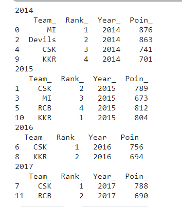
When you have to filter your data for a particular category or group then you can use group by function. To explain the group by function let’s create the new DataFrame, this data will contain the points of the IPL teams.
# import the pandas library
import pandas as pd
points_table = {'Team_':['MI', 'CSK', 'Devils', 'MI', 'CSK',
   'RCB', 'CSK', 'CSK', 'KKR', 'KKR', 'KKR', 'RCB'],
   'Rank_' :[1, 2, 2, 3, 3,4 ,1 ,1,2 , 4,1,2],
   'Year_' :[2014,2015,2014,2015,2014,2015,2016,2017,2016,2014,2015,2017],
   'Point_':[876,789,863,673,741,812,756,788,694,701,804,690]}
df = pd.DataFrame(points_table)
#Now group by the data according to the year
groupby_= df.groupby('Year_')
for team,group in groupby_:
   print(team)
   print(group)
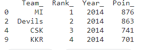
If you want to select a single group then you use the get_grouped() function.
print (groupby_.get_group(2014))
Here you can perform many aggregate functions.
Here you can perform some statistical operations on a set of data. let’s see the aggregate functions that are available in the Pandas package:
- count() – Count the number of non-null observation.
- sum() – sum of all the values / list
- min() – Minimum value
- max() – maximum value
- mean() – Arthmetic Mean
- median() – Arthmetic median()
- mode() – Mode
- std() – standard deviation
- var() – variance .
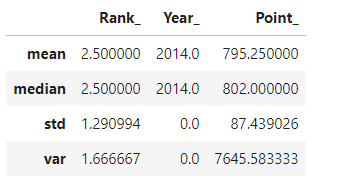
You can use the agg() function with the help of this you can perform several statistical computations at once.
Let’s implement them:-
import numpy as np
groupby_.get_group(2014).agg([np.mean,np.median,np.std,np.var ])
Min Max:
print("Maximum value : ",df.Point_.max())
print("Minimum value : ",df.Point_.min())

Count:
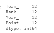
Count function is used to count the no-null values in the DataFrame.
df.count()
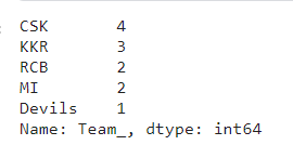
Value Counts:
You can use the value_counts() function which will give the count of each category.
df.Team_.value_counts()
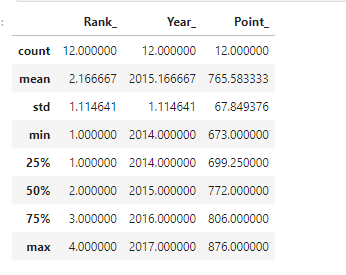
Describe:
If you want a complete statistical analysis of all the numerical values that are present in your dataset you can use the describe() function that will make your analysis easier.
df.describe()
Visualizations using Pandas Dataframe Operations
With the help of the Pandas library, you can also visualize the data in the form of different types of graphs such as line plots, bar charts, histograms, etc.
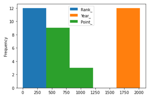
Histogram:
A histogram consists of rectangles whose area is proportional to the
frequency of a variable and whose width is equal to the class interval.
Dataframe.plot.hist(x,y,bins,**kwargs)
x,y:- Takes the coordinates of the x and y-axis.
bins:- Bins are the numbers that represent the intervals into which you want to group the source data.
**kwargs:- Takes the additional arguments.
df.plot.hist('Team_',bins=5)
Barplot:
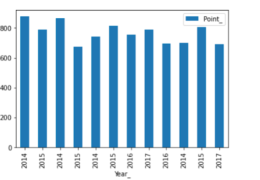
Bar graphs are the pictorial representation of data in the form of vertical and horizontal rectangular bars.
Dataframe.plot.bar(x,y,**kwargs)
x,y:- Takes the coordinates of the x and y-axis.
**kwargs:- Takes the additional arguments.
df.plot.bar(x='Year_',y='Point_' )
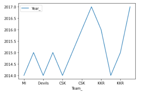
Line plot:
A line chart is a type of chart used to show information that changes over time.
Dataframe.plot.line(x,y,**kwargs)
x,y:- Takes the coordinates of the x and y-axis
**kwargs:- Takes the additional arguments.
df.plot.line(x='Team_',y='Year_')
Conclusion
In this article, you have seen three different DataFrames, first one is for the analysis of the data i.e how to perform various operations on rows and columns by using various functions that are present in the Pandas library while the other two DataFrames are about how to handle the missing values and how to use group by and apply an aggregate function on the DataFrame. At last, you have seen different types of plots such as histogram, barplot, etc., and how to visualize them by using the Pandas library.
Thanks for reading the article, please share if you liked this article.


