This article was published as a part of the Data Science Blogathon.
Introduction
Data Science associates with a huge variety of problems in our daily life. One major problem we see every day include examining a situation over time. Time series forecast is extensively used in various scenarios like sales, weather, prices, etc…, where the underlying values of concern are a range of data points estimated over a period of time. This article strives to provide the essential structure of some of the algorithms for solving these classes of problems. We will explore various methods for time series forecasts. We all would have heard about ARIMA models used in modern time series forecasts. In this article, we will thoroughly go through an understanding of ARIMA and how the Auto ARIMAX model can be used on a stock market dataset to forecast results.
Understanding ARIMA and Auto ARIMAX
- p is a particular order of the AR term
- q is a specific order of the MA term
- d is the number of differences wanted to make the time series stationary
”Auto Regressive” (AR) term is indicated by ”p”. This relates to the number of lags of Y to be adopted as predictors. ”Moving Average” (MA) term is associated with “q”. This relates to the number of lagged prediction errors that should conform to the ARIMA Model.
An Auto-Regressive (AR only) model has Yt that depends exclusively on its lags. Such, Yt is a function of the ‘lags of Yt’.

Furthermore, a Moving Average (MA only) model has Yt that depends particularly on the lagged forecast errors.

The time series differencing in an ARIMA model is differenced at least once to make sure it is stationary and we combine the AR and MA terms. Hence, The equation becomes:

We have continued operating through the method of manually fitting various models and determining which one is best. Therefore, we transpire to automate this process. It uses the data and fits several models in a different order before associating the characteristics. Nevertheless, the processing rate increases considerably when we seek to fit the complicated models. This is how we move for Auto-ARIMA models.
Implementation of Auto ARIMAX:
We will now look at a model called ‘auto-arima’, which is an auto_arima module from the pmdarima package. We can use pip install to install our module.
!pip install pmdarima
The dataset is available: https://www.kaggle.com/rohanrao/nifty50-stock-market-data.
df = pd.<a onclick="parent.postMessage({'referent':'.pandas.read_csv'}, '*')">read_csv("BAJAJFINSV.csv")
df.set_index("Date", drop=False, inplace=True)
df.head()
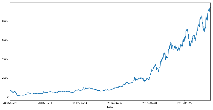
df.VWAP.plot(figsize=(14, 7))

We add some essential features like lag values of available numeric features widely accepted for time series problems. Considering we need to foretell the stock price for a day, we cannot use the feature values of the same day since they will be unavailable at actual inference time. We require to use statistics like the mean, the standard deviation of their lagged values. The three sets of lagged values are used, one previous day, one looking back seven days and another looking back 30 days as a proxy for last week and last month metrics.
df.reset_index(drop=True, inplace=True)
lag_features = ["High", "Low", "Volume", "Turnover", "Trades"]
window1 = 3
window2 = 7
window3 = 30

df_rolled_3d = df[lag_features].rolling(window=window1, min_periods=0)
df_rolled_7d = df[lag_features].rolling(window=window2, min_periods=0)
df_rolled_30d = df[lag_features].rolling(window=window3, min_periods=0)

df_mean_3d = df_rolled_3d.mean().shift(1).reset_index().astype(np.<a onclick="parent.postMessage({'referent':'.numpy.float32'}, '*')">float32)
df_mean_7d = df_rolled_7d.mean().shift(1).reset_index().astype(np.<a onclick="parent.postMessage({'referent':'.numpy.float32'}, '*')">float32)
df_mean_30d = df_rolled_30d.mean().shift(1).reset_index().astype(np.<a onclick="parent.postMessage({'referent':'.numpy.float32'}, '*')">float32)

df_std_3d = df_rolled_3d.std().shift(1).reset_index().astype(np.<a onclick="parent.postMessage({'referent':'.numpy.float32'}, '*')">float32)
df_std_7d = df_rolled_7d.std().shift(1).reset_index().astype(np.<a onclick="parent.postMessage({'referent':'.numpy.float32'}, '*')">float32)
df_std_30d = df_rolled_30d.std().shift(1).reset_index().astype(np.<a onclick="parent.postMessage({'referent':'.numpy.float32'}, '*')">float32)

for feature in lag_features:
    df[f"{feature}_mean_lag{window1}"] = df_mean_3d[feature]
    df[f"{feature}_mean_lag{window2}"] = df_mean_7d[feature]
    df[f"{feature}_mean_lag{window3}"] = df_mean_30d[feature]

    df[f"{feature}_std_lag{window1}"] = df_std_3d[feature]
    df[f"{feature}_std_lag{window2}"] = df_std_7d[feature]
    df[f"{feature}_std_lag{window3}"] = df_std_30d[feature]

df.fillna(df.mean(), inplace=True)

df.set_index("Date", drop=False, inplace=True)
df.head()
During boosting models, it is very beneficial to attach DateTime features like an hour, day, month, as appropriate to implement the model knowledge about the time element in the data. For time sequence models, it is not explicitly expected to pass this information, but we could do so, and we will discuss in this article so that all models are analysed on the exact identical set of features.
df.Date = pd.<a onclick="parent.postMessage({'referent':'.pandas.to_datetime'}, '*')">to_datetime(df.Date, format="%Y-%m-%d")
df["month"] = df.Date.dt.month
df["week"] = df.Date.dt.week
df["day"] = df.Date.dt.day
df["day_of_week"] = df.Date.dt.dayofweek
df.head()
The data is split in both train and test along with its features.
df_train = df[df.Date < "2019"]
df_valid = df[df.Date >= "2019"]

exogenous_features = ["High_mean_lag3", "High_std_lag3", "Low_mean_lag3", "Low_std_lag3",
                      "Volume_mean_lag3", "Volume_std_lag3", "Turnover_mean_lag3",
                      "Turnover_std_lag3", "Trades_mean_lag3", "Trades_std_lag3",
                      "High_mean_lag7", "High_std_lag7", "Low_mean_lag7", "Low_std_lag7",
                      "Volume_mean_lag7", "Volume_std_lag7", "Turnover_mean_lag7",
                      "Turnover_std_lag7", "Trades_mean_lag7", "Trades_std_lag7",
                      "High_mean_lag30", "High_std_lag30", "Low_mean_lag30", "Low_std_lag30",
                      "Volume_mean_lag30", "Volume_std_lag30", "Turnover_mean_lag30",
                      "Turnover_std_lag30", "Trades_mean_lag30", "Trades_std_lag30",
                      "month", "week", "day", "day_of_week"]
model = auto_arima(df_train.VWAP, exogenous=df_train[exogenous_features], trace=True, error_action="ignore", suppress_warnings=True)
model.fit(df_train.VWAP, exogenous=df_train[exogenous_features])

forecast = model.predict(n_periods=len(df_valid), exogenous=df_valid[exogenous_features])
df_valid["Forecast_ARIMAX"] = forecast
The most suitable ARIMA model is ARIMA(2, 0, 1) which holds the lowest AIC.
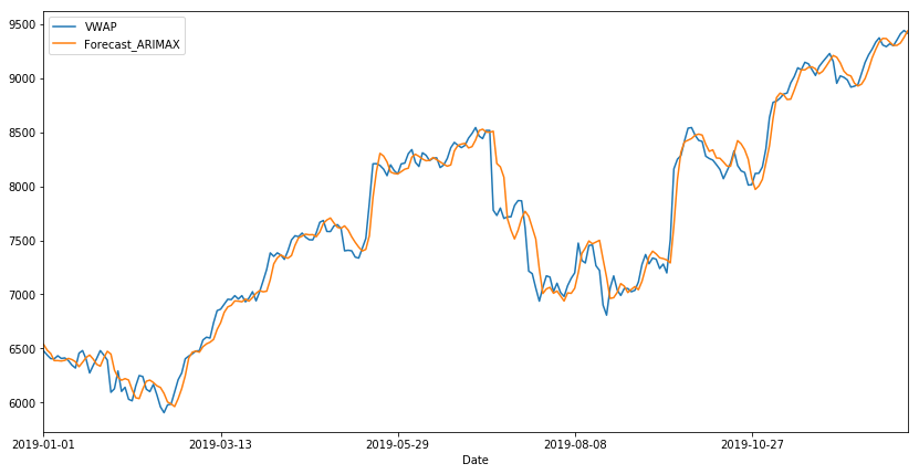
df_valid[["VWAP", "Forecast_ARIMAX"]].plot(figsize=(14, 7))

print("RMSE of Auto ARIMAX:", np.<a onclick="parent.postMessage({'referent':'.numpy.sqrt'}, '*')">sqrt(mean_squared_error(df_valid.VWAP, df_valid.Forecast_ARIMAX)))
print("nMAE of Auto ARIMAX:", mean_absolute_error(df_valid.VWAP, df_valid.Forecast_ARIMAX))
Conclusion:
In this article, we explored details regarding ARIMA and understood how auto ARIMAX was applied to a time series dataset. We implemented the model and got a score of about 147.086 as RMSE and 104.019 as MAE as the final result.
Reference:
- https://www.machinelearningplus.com/time-series/arima-model-time-series-forecasting-python/
- https://www.kaggle.com/rohanrao/a-modern-time-series-tutorial/notebook
About Me: I am a Research Student interested in the field of Deep Learning and Natural Language Processing and currently pursuing post-graduation in Artificial Intelligence.
Image Source
- Preview Image: https://medium.com/@fenjiro/time-series-for-business-a-general-introduction-50968346e660
Feel free to connect with me on:
- Linkedin: https://www.linkedin.com/in/siddharth-m-426a9614a/
- Github: https://github.com/Siddharth1698
The media shown in this article is not owned by Analytics Vidhya and are used at the Author’s discretion


This is a great post! I have been working with time series data for a while now and this post has really helped me to understand the concepts better.