How sklearn’s Tfidfvectorizer Calculates tf-idf Values

This article was published as a part of the Data Science Blogathon.

Overview

In NLP, tf-idf is an important measure and is used by algorithms like cosine similarity to find documents that are similar to a given search query.

Here in this blog, we will try to break tf-idf and see how sklearn’s TfidfVectorizer calculates tf-idf values. I had a hard time matching the tf-idf values generated by TfidfVectorizer and with the ones I calculated. The reason is that there are many ways in which tf-idf values are calculated, and we need to be aware of the method that TfidfVectorizer uses to calculate tf-idf. This will save a lot of time and effort for you. I spent a couple of days troubleshooting before I could realize the issue.

We will write a simple Python program that uses TfidfVectorizer to calculate tf-idf and manually validate this. Before we get into the coding part, let’s go through a few terms that make up tf-idf.

What is Term Frequency (tf)

tf is the number of times a term appears in a particular document. So it’s specific to a document. A few of the ways to calculate tf is given below:-

tf(t) = No. of times term ‘t’ occurs in a document

OR

tf(t) = (No. of times term ‘t’ occurs in a document) / (No. Of terms in a document)

OR

tf(t) = (No. of times term ‘t’ occurs in a document) / (Frequency of most common term in a document)

sklearn uses the first one i:e No. Of times a term ‘t’ appears in a document

Inverse Document Frequency (idf)

idf is a measure of how common or rare a term is across the entire corpus of documents. So the point to note is that it’s common to all the documents. If the word is common and appears in many documents, the idf value (normalized) will approach 0 or else approach 1 if it’s rare. A few of the ways we can calculate idf value for a term is given below

idf (t) =1 + log _e [ n / df(t) ]

OR

idf(t) = log _e [ n / df(t) ]

where

n = Total number of documents available

t = term for which idf value has to be calculated

df(t) = Number of documents in which the term t appears

But as per sklearn’s online documentation, it uses the below method to calculate idf of a term in a document.

idf(t) = log _e [ (1+n) / ( 1 + df(t) ) ] + 1 (default i:e smooth_idf = True)

and

idf(t) = log _e [ n / df(t) ] + 1 (when smooth_idf = False)

Term Frequency-Inverse Document Frequency (tf-idf)

tf-idf value of a term in a document is the product of its tf and idf. The higher is the value, the more relevant the term is in that document.

Python program to generate tf-idf values

Step 1: Import the library

from sklearn.feature_extraction.text import TfidfVectorizer

Step 2: Set up the document corpus

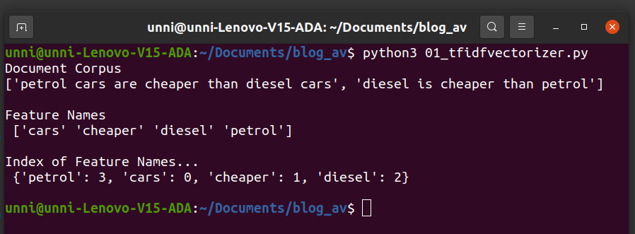
d1=”petrol cars are cheaper than diesel cars”

d2=”diesel is cheaper than petrol”

doc_corpus=[d1,d2]

print(doc_corpus)

Step 3: Initialize TfidfVectorizer and print the feature names

vec=TfidfVectorizer(stop_words='english')

matrix=vec.fit_transform(doc_corpus)

print("Feature Names n",vec.get_feature_names_out())

Step 4: Generate a sparse matrix with tf-idf values

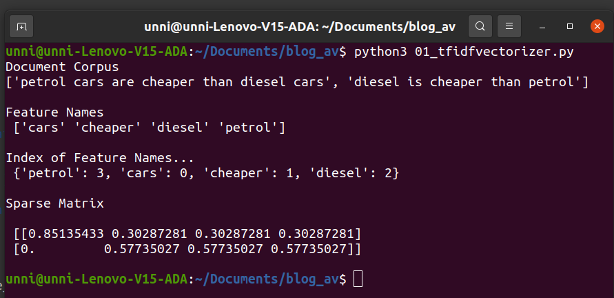
print("Sparse Matrix n",matrix.shape,"n",matrix.toarray())

Validate tf-idf values in the sparse matrix

To start with, the term frequency(tf) for each term in the documents is given in the above table.

Calculate idf values for each term.

As mentioned before , idf value of a term is common across all documents. Here we will consider the case when smooth_idf = True (default behaviour). So idf(t) is given by

idf(t) = log _e [ (1+n) / ( 1 + df(t) ) ] + 1

Here n=2 (no. Of docs)

idf(“cars”) = log _e (3/2) +1 => 1.405465083

idf(“cheaper”) = log _e (3/3) + 1 => 1

idf(“diesel”) = log _e (3/3) + 1 => 1

idf(“petrol”) = log _e (3/3) + 1 => 1

From the above idf values, we can see that as “cheaper”, “diesel” and “petrol” are common to both the documents , it has a lower idf value

Calculate tf-idf of the terms in each document d1 and d2.

For d1

tf-idf(“cars”) = tf(“cars”) x idf (“cars”) = 2 x 1.405465083 => 2.810930165

tf-idf(“cheaper”) = tf(“cheaper”) x idf (“cheaper”) = 1 x 1 => 1

tf-idf(“diesel”) = tf(“diesel”) x idf (“diesel”) = 1×1 => 1

tf-idf(“petrol”) = tf(“petrol”) x idf (“petrol”) = 1×1 => 1

For d2

tf-idf(“cars”) = tf(“cars”) x idf (“cars”) = 0 x 1.405465083 => 0

tf-idf(“cheaper”) = tf(“cheaper”) x idf (“cheaper”) = 1 x 1 => 1

tf-idf(“diesel”) = tf(“diesel”) x idf (“diesel”) = 1×1 => 1

tf-idf(“petrol”) = tf(“petrol”) x idf (“petrol”) = 1×1 => 1

So we have the sparse matrix with shape 2 x 3

[

[2.810930165                           1                     1                    1]

[0                                                1                     1                     1]

]

Normalize tf-idf values

We have one final step. To avoid large documents in the corpus dominating smaller ones, we have to normalize each row in the sparse matrix to have the Euclidean norm.

First document d1

2.810930165 / sqrt( 2.810930165 ² + 1² + 1² + 1²) => 0.851354321

1 / sqrt( 2.810930165² + 1² + 1² + 1²) =>  0.302872811

1 / sqrt( 2.810930165² + 1² + 1² + 1²) => 0.302872811

1 / sqrt( 2.810930165² + 1² + 1² + 1²) => 0.302872811

Second document d2

0 / sqrt(0 ²   + 1² + 1² + 1²) => 0

1 / sqrt(0²  + 1² + 1² + 1²)=> 0.577350269

1/ sqrt(0²  + 1² + 1² + 1²) => 0.577350269

1 / sqrt(0²  + 1² + 1² + 1²) => 0.577350269

This gives us the final normalized sparse matrix

[

[0.851354321         0.302872811        0.302872811        0.302872811]

[0                               0.577350269       0.577350269        0.577350269]

]

And the above sparse matrix that we just calculated matches the one generated by TfidfVectorizer from sklearn.

Conclusion from tf-idf values

Below were the tf values of both documents d1 and d2

(i) In the first document d1, the term “cars” is the most relevant term as it has the highest tf-idf value (0.851354321)

(ii) In the second document d2, most of the terms have the same tf-idf value and have equal relevance. 

The complete Python code to build the sparse matrix using Tfidfvectorizer is given below for ready reference.

from sklearn.feature_extraction.text import TfidfVectorizer

doc1="petrol cars are cheaper than diesel cars"

doc2="diesel is cheaper than petrol"

doc_corpus=[doc1,doc2]

print(doc_corpus)

vec=TfidfVectorizer(stop_words='english')

matrix=vec.fit_transform(doc_corpus)

print("Feature Names n",vec.get_feature_names_out())

print("Sparse Matrix n",matrix.shape,"n",matrix.toarray())

Closing Notes

Unnikrishnan C S 03 Nov 2021