Implementing Particle Swarm Optimization using Python

This article was published as a part of the Data Science Blogathon.

Introduction

There are multiple ways that one can take to either minimize or maximize any function so that the optimal value can be found out. You can find several optimisation solutions on the internet but in the end, no one solution is the best for all. Everyone has its own advantage and disadvantages. The one that we are going to discuss here is the PSO or the Particle Swarm Optimization. You can also say that it is a field of optimisation which belongs to the nature-inspired way of computing. It is a type of algorithm which searches for the optimal solution in a definite space in a straightforward manner.

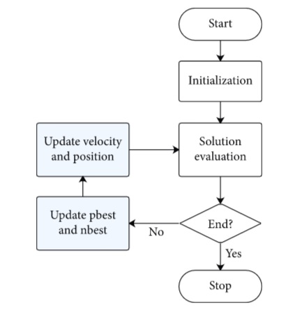
The solution works by the logic where a candidate solution is worked upon to make it better by a specific measure of quality and then the operation is performed iteratively until a better solution is not available and thus reaching an optimal state itself. The language here will be Python and we will see a hands-on implementation of it using a python package “PySwarms”. We will cover the following topics here :

1. PSO: Particle Swarm Optimization
2. The inner workings
3. Variants or types of PSO
4. Implementing PSO with PySwarms

What is Particle Swarm Optimization (PSO)?

In the 1990s there were a number of studies conducted on the topic of the social behavior of animal clusters. These research studies concluded with one of the learnings being that some animal groups such as birds or fishes are able to pass on their knowledge or communicate with others in the group. This sometimes helped them survive attacks or get an advantage over other animal groups when evading predators. Based on all of this research, Kennedy and Eberhart proposed a PSO algorithm. In 1995, this PSO algorithm was proposed as a metaheuristic algorithm. This algorithm worked to optimise nonlinear continuous functions based on the concept of animal swarm intelligence exhibited in flocks and shoals.

The studies concluded that there was knowledge or wisdom sharing amongst animals that helped them get insight into a situation they haven’t faced before. In simpler words, finding food or evading prey becomes easy when all the birds of a flock share their observations and knowledge. The optimal solution hence becomes easier to pin down with swarm intelligence.

Inner working of Particle Swarm Optimization

Swarm behaviour can be of two types. First is the exploratory behaviour where animals seek their object in a larger solution space. Second is the exploitative behaviour where swarm intelligence helps them search a smaller more optimum area. PSOs and their parameters are mostly designed to find an optimum balance between exploration and exploitation. This ensures a good rate of convergence to the optimum.

2.1 Convergence of Particle Swarm Optimization

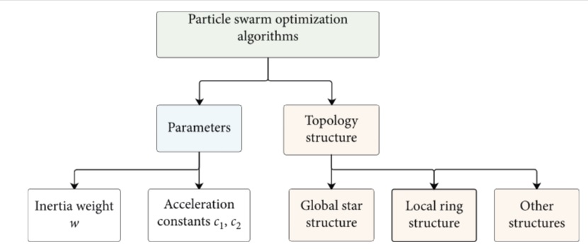
In a PSO convergence, it does not matter how a swarm will operate but the convergence to a specific local optimum when various personal bests which let’s say P or the best-known position of the swarm or also known as G will reach a local optimum for the problem. The ability which a PSO algorithm has so that it can exploit and explore can get affected by the topology structure. So for different structures, the algorithm can converge in a different manner because of the shape of the topology which is generally either a local ring or a global star. The topology structure defines the factors like searching, information sharing, speed, and even the direction in which each particle should follow.

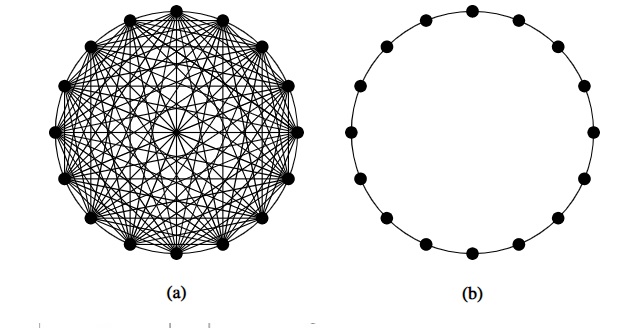
A PSO which has a global star structure where all particles are connected with each other has one benefit of the shortest average distance but a local ring structure where one particle is connected with the two nearest ones has the highest average distance in the whole swarm as shown in the above image. The figure on the left is the global star structure whereas the left one is the local ring structure. Each group consists of 16 particles and you can see why the average distance differs for both cases.

2.2 Adaptive mechanism

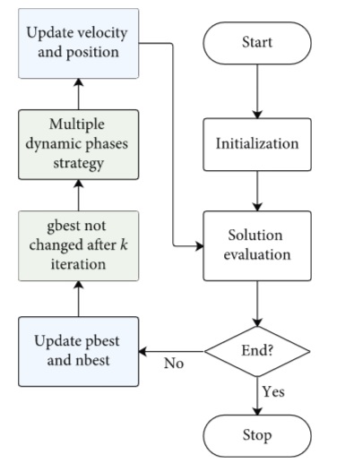
In an Adaptive mechanism, one can implement it with the required trade-off between convergence and divergence or exploitation and exploration. An APSO or Adaptive Particle Swarm Optimisation can outperform a regular PSO. With a faster convergence time, an APSO could also execute any global search across the whole search space.

Variants of Particle Swarm Optimization

PSO algorithms can be of different types, even simple ones. The particles and velocities can be initiated in different ways. Update the Swarm and then set values for Pi and G and so forth.

3.1 Gradient Particle Swarm Optimization

We can construct gradient-based PSOs by combining the efficiency of the PSO at exploring many local minimums with the gradient-based local search algorithms. This helps us to accurately calculate a local minimum. The PSO algorithm can be used for gradient-based PSO also where several local minima are discovered along with a deep basin of attraction for a deep local minimum. The deep minimum can then be confirmed using the local gradient-based search techniques.

3.2 Hybrid Particle Swarm Optimization

In order to increase and make the optimization process better, newer and more advanced types of PSO variations are being tested and used and are an ongoing field of study. A Hybrid PSO is where a normal PSO is combined with another optimization technique which helps to make it better. One example is Biogeography based optimization while also implementing an effective learning mechanism that will improve the existing PSO and enhance it.

4. Implementing Particle Swarm Optimization using PySwarms

As the name suggests, PySwarms is a python based tool that helps with swarm optimisation. Researchers, practitioners, and students alike use this tool in order to apply the PSO algorithm using a high-level interface. PySwarms is the best tool to integrate swarm optimisation with basic optimization.

This tool allows you to implement and use a number of many-particle swarm optimisation techniques. It’s also extremely user-friendly and adaptable to different projects. Your optimisation problem can also benefit from the support modules.

Now we will move on to using a global best optimizer using PySwarm’s functional API which is “pyswarms.single.GBestPSO” . We will plot it in both 2D and 3D manner.

You can install PySwarm by the following commands :

!pip install pyswarms

Now we will begin by importing some modules first :

Code :

# Import all the modules
import numpy as np
# Importing PySwarms
import pyswarms as ps
from pyswarms.utils.functions import single_obj as fx
import matplotlib.pyplot as plt
from pyswarms.utils.plotters import plot_contour, plot_surface
from pyswarms.utils.plotters.formatters import Designer
from pyswarms.utils.plotters.formatters import Mesher

After importing them all, we will begin with improving our sphere function, you can put any arbitrary settings to begin within our optimizer. The main three steps here are :

1. 1. Set the hyperparameters to configure the swarm as a dictionary
2. 2. To create the instance of an optimizer, pass the dictionary with all the relevant input parameters
3. 3. The best cost and position in a variable can be saved by invoking the “optimize()” function.

#import numpy as np
# Importing PySwarms
import pyswarms as ps
from pyswarms.utils.functions import single_obj as fx
#import matplotlib.pyplot as plt
#from pyswarms.utils.plotters import plot_contour, plot_surface
#from pyswarms.utils.plotters.formatters import Designer
#from pyswarms.utils.plotters.formatters import Mesher

# Set-up all the hyperparameters
options = {'c1': 0.5, 'c2': 0.3, 'w':0.9}
# Call an instance of PSO
optimizer = ps.single.GlobalBestPSO(n_particles=10, dimensions=2, options=options)
# Perform the optimization
cost, pos = optimizer.optimize(fx.sphere, iters=1000) 

4.1 Now on Visualizing the function

PySwarm already comes with various tools which will help you to visualise the behaviours of the swarm. These behaviours are constructed on the top of matplotlib which results in high customizable charts and user friendly too. There are also animation methods which are  “plot_contour()” and “plot_surface()” methods. These methods plot the particle in a 2D and 3D space respectively. To plot the sphere function, we need to add a specific function called mesh function into our swarm.

These help to visualise the particles graphically. We have already imported the “Mesher” class which helps us to achieve this. The “pyswarms.utils.plotters.formatters” module has many different formats so that you can customize the plots. Apart from Mesher, there is a “Designer” class that modifies the figure size, font size, and more along with an animator class for setting repeats and animation delays.

Code for 2D Plot :

m = Mesher(func=fx.sphere)
animation = plot_contour(pos_history=optimizer.pos_history,
                         mesher=m,
                         mark=(0,0))

Output :

#Code for 3D Plot :
# The preprocessing
pos_history_3d = m.compute_history_3d(optimizer.pos_history)
# Adjusting the figure
d = Designer(limits=[(-1,1), (-1,1), (-0.1,1)], label=['x-axis', 'y-axis', 'z-axis'])
animation3d = plot_surface(pos_history=pos_history_3d, # The cost_history that we computed
                           mesher=m, designer=d,       # Various Customizations
                           mark=(0,0,0))               # Mark the minima

Output :

Note: Support for .gif will soon be added and hence youtube upload for now. The First 10 seconds of the video are essential, the rest is not much. The collab notebook link is given below :

Conclusion

So in this post, we have seen the theory and how a PSO works and explored the inner mechanism. We saw some of its variants and how it has been used in various domains and communities. Last but not least we also implemented a small python based swarm of our own. Feel free to text me if you face any issues or run into any problems.

Ankita Roy

Class of 2022 IT, Open to full-time/internships

[email protected]

Links to images :

1. Image 1 – https://www.hindawi.com/journals/ddns/2021/8378579/fig1/
2. Image 2 – https://www.hindawi.com/journals/ddns/2021/8378579/fig2/
3. Image 3 – https://www.hindawi.com/journals/ddns/2021/8378579/fig1/
4. Image 4: https://www.hindawi.com/journals/ddns/2021/8378579/fig5/
5. https://unsplash.com/photos/b7MZ6iGIoSI
6. https://unsplash.com/photos/qvIeCwqxzU4