Polish Up your ML model!

This article was published as a part of the Data Science Blogathon.

Introduction

In this article, we will be discussing various ways through which we can polish up or fine-tune our machine learning model. We will be using the Housing Dataset for understanding the concepts.

Before we get started let’s get a quick view of the dataset we are about to work on: California housing Prices 

 

Let’s take a look at the first five rows using the Dataframe’s head method.

housing.head()

Here we see that each row is representing one district.

In total, there are ten attributes:

1. longitude
2. latitude
3. housing_median_age
4. total_rooms
5. total_bedrooms
6. population
7. households
8. median_income
9. median_house_value
10. Ocean_proximity

Let us go ahead and use the info method to get a piece of quick information about the data.

housing.info()

Here we can see that there are 20640 instances available in the dataset, which is a little bit less from a machine learning perspective, but good enough to get started. Now you might have noticed the total bedrooms attribute because it only has 20433 values which means the rest of 207 values are null.

Now we can see that ocean proximity is the only attribute that is non-numerical in nature, its type is an object, which means it could be any type of python object but as this data is loaded from a CSV file, it must be a text. Let’s take a look at the ocean proximity attribute.

housing['ocean_proximity'].value_counts()

As we all know that this is a categorical attribute, you can check out my previous blog Cook the data for your machine learning algorithm here in which I have explained how to deal with both missing values as well as categorical attributes in point number 3 which is Text and categorical attributes.

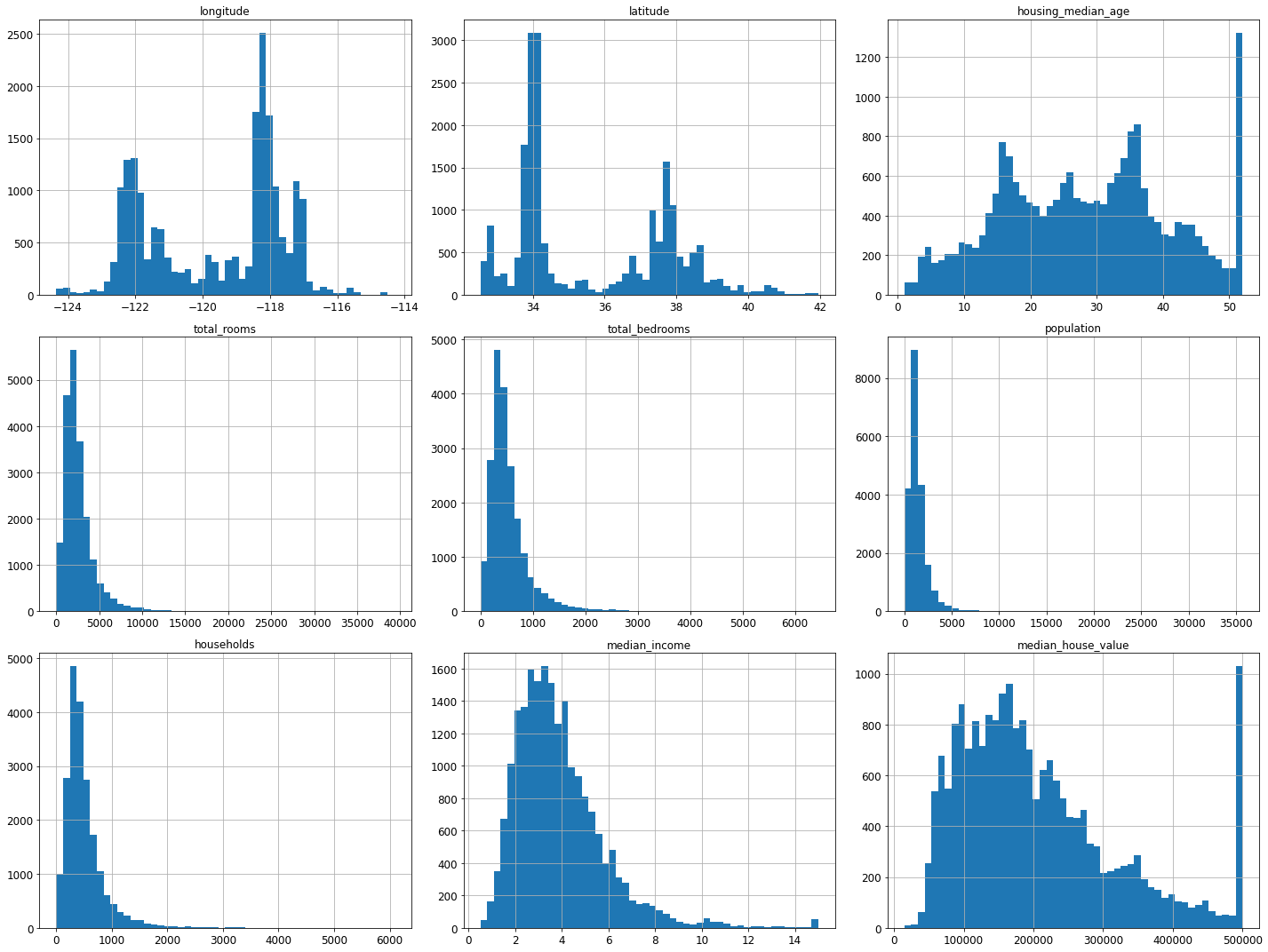
Lastly, to get a feel of what type of data we are dealing with let’s go ahead and plot a histogram for each numerical attribute.

%matplotlib inline
import matplotlib.pyplot as plt
housing.hist(bins=50,figsize=(25,30))
plt.show()

Hopefully, now you have a better intuition of what kind of data we are working with. Now without any further ado let’s get started with fine-tuning.

What does Fine-tuning our model mean?

In simple words, fine-tune model is just like rotating the antenna of television until we get a clear picture. Just like that here we have to adjust our model’s hyperparameters to achieve maximum accuracy.

Assuming you have a list of promising models. Now, all we need to do is fine-tune them. Let’s look at a couple of ways we can do that.

1. Grid Search:

One thing you could do is, you can fiddle with the hyperparameters manually until you find a great combination of hyperparameters values. But this task would be very tedious, may take a lot of time, and also you might not be able to explore as many combinations.

Here comes, Sckit-learn’s Grid Search CV in the picture to help you. All you need to do is tell it which hyperparameters you want it to choose and with what values you want it to experiment with and it will use cross-validation to evaluate all possible combinations of hyperparameter values.

Let’s see the implementation:

from sklearn.model_selection import GridSearchCV
from sklearn.ensemble import RandomForestRegressor

para_grid = [

    {'n_estimators':[2,10,30],'max_features':[2,4,6,8]},

    {'bootstrap':[False],'n_estimators':[2,10],'max_features':[2,4,6]},

] 

forest_reg = RandomForestRegressor()
Grid_search = GridSearchCV(forest_reg,para_grid,cv=10,scoring='neg_mean_squared_error',return_train_score=True)
Grid_search.fit(prepared,labels)

Whenever while working on the ML model, if you have no idea what values of hyperparameters to use, go with consecutive power of 10.

Here what this para_grid will do is, it will tell scikit-learn to first evaluate all 3*4 = 12 combinations of n_estimator and max_features hyperparameter values specified first after that it tries all 2*3 = 6 combinations of hyperparameter values specified second, in second bootstrap value is set to false instead of true (which is the default value of this hyperparameter).

Scoring is set to ‘neg_mean_absolute_error‘:  this is a negative version of the mean absolute error, where values closer to zero represent less prediction error by the model.

Hence grid search will try all 12 + 6  = 18 combinations of RandomForestRegressor hyperparameters values, also it will train each model 10 times Since we are using 10 fold cross-validation. Therefore, in total there will be 18*10 = 180 rounds of training! It will be time-consuming but once when done you will end up with the best combination of hyperparameter values.

Here, we can see that 8 and 30 were the maximum values that were specified, so we can try searching again with higher values, the accuracy may improve.

In this example, we obtained the best solutions by initializing max_features hyperparameter to 8 and n_estimators hyperparameter to 30. The RMSE score by settings these parameters would for sure be better than the score with default parameters.

2. Randomized Search:

Image 4

The grid search technique is appropriate whenever you’re trying to explore a few combinations of hyperparameters. But if you want to search and explore a lot of hyperparameter combinations is preferable that you use a randomized search technique for it. This technique is almost as similar as grid search, the only difference is that instead of trying all possible combinations, it evaluates random numbers combinations by setting random values for each hyperparameter.

The main benefits of this approach are:

1.  Let’s say you run a search for 500 iterations, so this approach will explore 500 different values for each hyperparameter, instead of just a few in case of grid search.
2. All you got to do is simply set the number of iterations, and you will have more control over the computing budget you want to allocate to hyperparameter search.

3. Ensemble Method:

Image 5

Another way through which you could fine-tune of machine learning model is by combining the models that perform best. This group of best models also known as an ensemble will for sure perform better than the best individual model(as we all know that Random forests perform better than individual decision trees because Random Forest, in simple terms is just a bunch of decision trees), especially when they make different errors.

We will look at this interesting topic in detail in the upcoming blogs. Stay TUNED!

4. Analysis of our Best Models:

Image 6

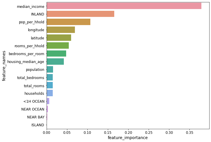
There may be times when you might gain good intuition on your problem by scrutinizing your best models. For better understanding let’s take an example, here random forest regressor has the ability to indicate the importance of each attribute for better predictions:

We will be using the same grid search that we have initialized in the first point here.

feature_importances = grid_search.best_estimator_.feature_importances_
feature_importances

Let’s go ahead and display all these scores next to their corresponding attributes:

 

With this data, we can easily make decisions of dropping less useful attributes and keep the important ones.

While doing all this you should also look at whether your models are making some specific errors or not, if yes try to understand why it is happening and counter this with adding some features, getting rid of the unnecessary ones, removing outliers, etc.

WARNING!

 

Image 7

Whenever you are fine-tuning your model by twerking your hyperparameters, beware that if you did a lot of hyperparameter tuning the performance will slightly degrade because after that your model will end up fine-tuned to perform well on your validation data and may or may not perform well on datasets your model has never encountered before. Whenever this kind of scenario exists, you need to resist the temptations of twerking your hyperparameters. These kinds of improvements may benefit while working with test data but will be unlikely to generalize to new data.

Image Source-

• Image 1: https://www.google.com/url?sa=i&url=https%3A%2F%2Funsplash.com%2Fs%2Fphotos%2Fshoe-polish&psig=AOvVaw30NAKICDUtYRqhyNmztd-A&ust=1636211866945000&source=images&cd=vfe&ved=0CAsQjRxqFwoTCPCyy6vCgfQCFQAAAAAdAAAAABAD
• Image 2: https://www.google.com/url?sa=i&url=https%3A%2F%2Fwww.kaggle.com%2Fharrywang%2Fhousing&psig=AOvVaw0uyiz6huei8zbjgQh4F4Xh&ust=1636716794908000&source=images&cd=vfe&ved=0CAsQjRxqFwoTCIDq566bkPQCFQAAAAAdAAAAABAD
• Image 3: https://www.google.com/url?sa=i&url=https%3A%2F%2Funsplash.com%2Fs%2Fphotos%2Fmagnifying-glass&psig=AOvVaw11aYVsP6pLnWGlf1U8trxi&ust=1636215241727000&source=images&cd=vfe&ved=0CAsQjRxqFwoTCLjer_jOgfQCFQAAAAAdAAAAABAD
• Image 4: https://www.google.com/url?sa=i&url=https%3A%2F%2Fwww.istockphoto.com%2Fphotos%2Fsherlock-holmes&psig=AOvVaw2YgUwQyVY_8rpYM4ZMZXe2&ust=1636260157977000&source=images&cd=vfe&ved=0CAsQjRxqFwoTCKjRraj2gvQCFQAAAAAdAAAAABAd
• Image 5: https://www.google.com/url?sa=i&url=https%3A%2F%2Fwww.capitalfm.com%2Fnews%2Ftv-film%2Ffriends%2Ffriends-plot-hole-monica-chandler%2F&psig=AOvVaw3V_Gki4Lwq1XucGfHP_Lxg&ust=1636630480062000&source=images&cd=vfe&ved=0CAsQjRxqFwoTCIjn4ebZjfQCFQAAAAAdAAAAABAJ
• Image 6: https://www.google.com/url?sa=i&url=https%3A%2F%2Funsplash.com%2Fs%2Fphotos%2Fdata-analysis&psig=AOvVaw3u2qK2WDBddhoAMCkvy3_k&ust=1636630612104000&source=images&cd=vfe&ved=0CAsQjRxqFwoTCODg36XajfQCFQAAAAAdAAAAABAD
• Image 7: https://www.google.com/url?sa=i&url=https%3A%2F%2Fgetyarn.io%2Fyarn-clip%2Fd0232b8d-0f80-47e2-ab72-0fbea1591bff%2Fgif&psig=AOvVaw1T1e0hhiHgXOY_e_NRXZ6K&ust=1636645870844000&source=images&cd=vfe&ved=0CAsQjRxqFwoTCMCn8JCTjvQCFQAAAAAdAAAAABAD

Conclusion:

So to wrap up let’s go through the things that we have learned in this article. Today, we went from what does fine-tuning mean? and several ways through which we can achieve it. Also, do check out other blogs, articles, and videos to get a tighter grip on this concept as it’s a vital one.

Stay tuned!!

Check out my other blogs here.

I hope you enjoyed reading this article, if you found it useful, please share it among your friends on social media too. For any queries and suggestions feel free to ping me here in the comments or you can directly reach me through email.

Connect me with on LinkedIn

Email: [email protected]

Thank You!

Karan