This article was published as a part of the Data Science Blogathon.
A brief introduction to transfer learning
The most pervasive problems in machine learning are related to data: it can be either insufficient, or low-quality. One obvious solution to this set of problems is to acquire more and better data. However, these two often do not go together. We have to sacrifice quality for quantity or vice versa. Fortunately, there is a more innovative solution: transfer learning.
Transfer learning is a method of reusing an already trained model for another task. The original training step is called pre-training. The general idea is that, pre-training “teaches” the model more general features, while the latter final training stage “teaches” it features specific to our own (limited) data.
Transfer learning is especially useful in fields such as medicine, where data shortage remains a permanent problem. Various CNN models pre-trained on ImageNet data have proven successful in different medical tasks [7]. All it takes is a few lines of code to transfer them to medical data.
In this article, we are going to learn how to do this with TensorFlow, the most widely used Deep Learning platform in the world (as of 2021). Before we delve into the code, let’s have a quick recap of TensorFlow and Keras API that powers it.
Tensorflow and Keras API

TensorFlow is an end-to-end platform that enables building and deploying ML models. We are only interested in building models, not deploying them, and for that, we need to use Keras. Keras is an API designed for “human beings, not machines,” to quote themselves. That’s to say, Keras is designed for coders like us who want to build custom models. Its simple and easy-to-remember syntax makes it almost addictive.
While Keras API itself is available as a stand-alone Python library, it is also available as part of the TensorFlow library. Using tensorflow.keras is recommended over Keras itself, as it is maintained by the TensorFlow team, which ensures consistency with other TensorFlow modules.
Case study: Binary Image Classification
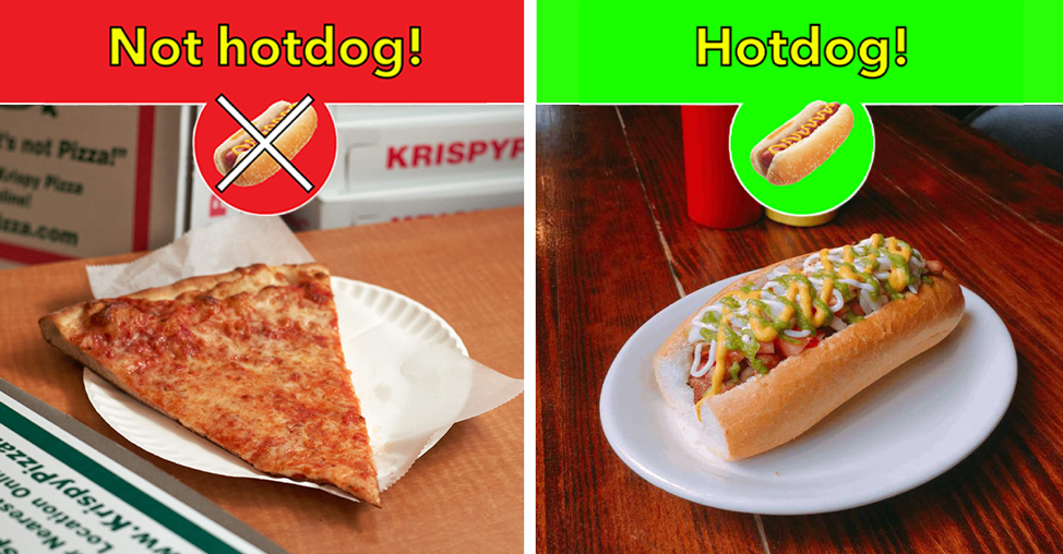
As a first example, we will try binary image classification. Our dataset will be Hot Dog – Not Hot Dog from Kaggle [6] and we will try to predict — you guessed it — whether the given image is a hot dog or not.
For this, we will use the ResNet50 model that was pre-trained on ImageNet dataset. ResNet refers to a set of architectures that uses residual connections to solve the degradation problem — degradation of accuracy, that is.
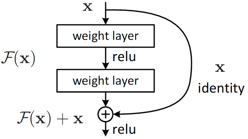
The figure above depicts residual mapping. This connection skips one (or more) layers and performs identity mapping, F(x) + x. This minor tweak in network architecture has had tremendous success against the degradation problem [8]. As a result, ResNet architectures can be as deep as 1000 layers. Our specific model choice, ResNet50 is a relatively shallow example. You can see its overall architecture in the following figure:
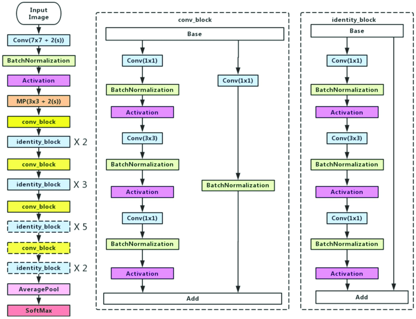
There are alternatives to ResNet family: MobileNets, Inception, etc. have also proven successful in image classification. You can also choose one of these, or an entirely different network and perform transfer learning on that.
I will work on Google Colab, which I recommend for anyone whose computer is not up to the task, although it is not a strict requirement. You can run the code in any environment you choose, including Jupyter Notebook or PyChram.
Let’s go through the process step by step.
Set up the environment for Transfer learning with TensorFlow
Note: This step may vary depending on your preferred environment.
# Upload the kaggle API key
from google.colab import files
files.upload()
! mkdir ~/.kaggle
! cp kaggle.json ~/.kaggle/
! chmod 600 ~/.kaggle/kaggle.json
# Install the kaggle package
! pip install -q kaggle
# Download the dataset from Kaggle
! kaggle datasets download -d dansbecker/hot-dog-not-hot-dog
# Import the necessary packages
import tensorflow as tf
from tensorflow import keras
from PIL import Image
import os
import numpy as np
Load the data for Transfer learning with TensorFlow
# Unzip the downloaded zip file
!unzip /content/hot-dog-not-hot-dog.zip
# Let's check size of images
for image in list(os.walk("/content/train/not_hot_dog"))[0][2]:
  a = Image.open(f"/content/train/not_hot_dog/{image}")
  print(np.asarray(a).shape)
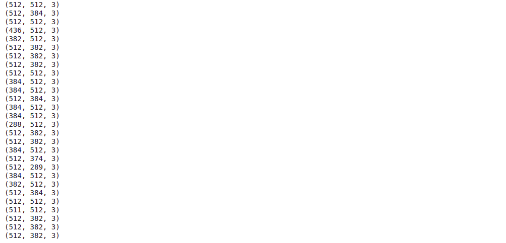
This is only a part of the output, but we can already see that image sizes are not constant. ImageDataGenerator deals with this sort of problems, among many other things.
Image data is essentially an array of numbers. Colored images are represented by a combination of three 2D matrices. Each of these matrices are composed of values between 0 and 255 (this may vary). Three of these values combined (each from one matrix) represent coIour of the pixel. In our case, our images have the shape of (512, 512, 3). That’s to say, we have 512*512=262144 pixels and 3 channels. (As we already said, not all of them conform to 512*512 size, but we will deal with it.)
# Create ImageDataGenerator objects
train_datagen = tf.keras.preprocessing.image.ImageDataGenerator()
test_datagen = tf.keras.preprocessing.image.ImageDataGenerator()
# Assign the image directories to them
train_data_generator = train_datagen.flow_from_directory(
    "/content/train",
    target_size=(512,512)
)
test_data_generator = train_datagen.flow_from_directory(
    "/content/test",
    target_size=(512,512)
)
ImageDataGenerator object will generate the data in batches for our model when necessary. This allows us to work directly with data stored on hard disk, without overloading the RAM. train_data_generator and test_data_generator will be passed as arguments to x and validation_data parameters, respectively. Since ImageDataGenerator obtains the classes from folder names, we do not need the y parameter. (If you try to pass an argument to y, Python will throw an error. )
Now that our train and test data are set, we can build and train our model.
Build the Transfer Learning Model with TensorFlow
At first, we will load the Keras implemetation of ResNet50 model.
resnet_50 = tf.keras.applications.resnet50.ResNet50(include_top=False, weights='imagenet')
resnet_50.trainable=False
include_top=False ensures that the last layer of ResNet50 model will not be loaded. weights=’imagenet’ loads the ImageNet weights. If we set weights=None, then the weights would be initialized randomly (in this case, we would not be performing transfer learning). By setting the trainable attribute to False, we ensure that the original (ImageNet) weights of the model will remain constant.
We need a binary classifier, but ResNet50 has more than 2 nodes in the final layers. This means that we have to add the final layer manually. I have used functional API, which can be challenging if you are a beginner TensorFlow user. (In that case, I suggest you use the Sequential API, which has more straightforward syntax.)
inputs = keras.Input(shape=(512,512,3))
x = resnet_50(inputs)
x = keras.layers.GlobalAveragePooling2D()(x)
outputs = keras.layers.Dense(2, activation="softmax")(x)
model = keras.Model(inputs=inputs, outputs=outputs, name="my_model")
model.compile(optimizer="Adam", loss="binary_crossentropy", metrics=["accuracy"])
model.summary()
In these lines, we define our input, pass it to the resnet_50 model that we defined earlier, pass its output to a Global Average Pooling layer, pass its output to a Dense layer with nodes (for two classes). Activation function has to be softmax in this case. Sum of the values of the softmax output vector is always equal to 1. For two nodes (each node represents a class), we have x1 + x2 = 1, where x1 and x2 represent class probabilities. (Otherwise, we can have 1 node and sigmoid activation function). After all these, we need to compile the model by selecting an optimizer and a loss function. We can also add which metrics to measure during the training process. Finally, we can train our model.
model.fit(train_data_generator, validation_data=test_data_generator, epochs=5)

We are done with the transfer learning part. Optionally, you can fine-tune the model to get better results.
Final notes
In this article, we learned how to implement transfer learning with help of TensorFlow. Transfer learning is a powerful approach that allows us to overcome data shortage. However, it is not a silver bullet; there are cases when working with whatever data we have makes more sense and yields better results. And it has alternatives. Data augmentation is a common one. Of course, these two are not exclusive. Different approaches can be (often are) combined to solve the data problem.
References
[1] https://www.tensorflow.org/tutorials/images/transfer_learning#create_the_base_model_from_the_pre-trained_convnets
[2] https://www.tensorflow.org/api_docs/python/tf/keras/applications/resnet50/ResNet50
[3] https://www.tensorflow.org/api_docs/python/tf/keras/preprocessing/image/ImageDataGenerator
[4] https://www.tensorflow.org/api_docs/python/tf/keras/Model
[5] https://www.kaggle.com/general/74235
[6] https://www.kaggle.com/dansbecker/hot-dog-not-hot-dog
[7] https://www.ncbi.nlm.nih.gov/pmc/articles/PMC5583361/
[8] https://arxiv.org/abs/1512.03385
Images
1 – https://www.toptal.com/machine-learning/tensorflow-machine-learning-tutorial
2 – https://github.com/tensorflow/tensorflow
3 – https://netbasequid.com/blog/social-analytics-hotdog/
4 – https://neurohive.io/en/popular-networks/resnet/
5 – https://www.researchgate.net/figure/Left-ResNet50-architecture-Blocks-with-dotted-line-represents-modules-that-might-be_fig3_331364877
6 – https://colab.research.google.com/drive/1pYVZtULa3pKncA7C2umg9LA5tqOCCos3?usp=sharing
7 – https://colab.research.google.com/drive/1pYVZtULa3pKncA7C2umg9LA5tqOCCos3?usp=sharing

