Custom Object Detection on the browser using TensorFlow.js

This article was published as a part of the Data Science Blogathon

What is object detection?

Cf the many Computer Vision cognitive application, object detection is one of the highly used techniques to identify and locate objects in images and videos.

As the name suggests – ‘Computer Vision’, is the ability for computers to acquire human-like vision to see and identify objects. Object Detection can be considered as image recognition with some advanced features. Not only does the algorithm recognize/identify the objects in images/videos, but also localizes them. In other words, a bounding box is created around the object in the image or video frames.

 

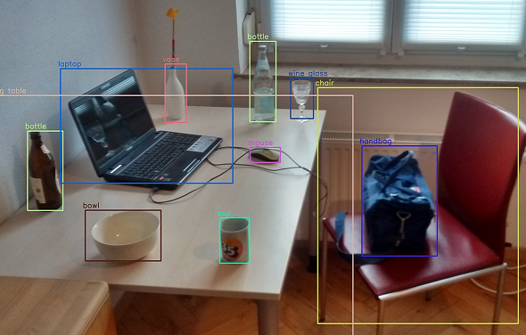
Various Object Detection algorithms

Following are some popular algorithms used for object detection:

• R-CNN: Region-based Convolutional Neural Networks
• Fast R-CNN: Fast Region-based Convolutional Neural Networks
• Faster R-CNN: Faster Regional-based Convolutional Networks
• YOLO: You Only Look Once
• SSD: Single Shot Detector

Each of the algorithms has its own pros and cons. The details of how these algorithms work are beyond the scope of this article. However, if you wish to learn more about them, you may refer to the following link:

https://en.wikipedia.org/wiki/Object_detection#Methods

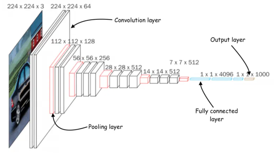
The architecture of a Convolutional Neural Network [Image source: https://bdtechtalks.com/2021/06/21/object-detection-deep-learning/]

As I pen down this article, I remember the good old days when I used to come home from school in the evening and switch on the TV to watch my favorite cartoons. I am sure we all loved watching cartoons. So, how about reliving those days again? Didn’t understand? Let me explain.

Today, we’ll learn how to create an end-to-end custom object detection web application using TensorFlow.js. We’ll train the model on a custom dataset and deploy it on the browser as a full-fledged web application. If you’re excited to build your own object detection model, what are you waiting for? Let’s dive in.

I’ll be creating a model that detects cartoons in real-time on the browser. Feel free to choose your own dataset because the overall process remains the same.

Create a dataset

The first step is to collect images of the objects you want to detect. Some of my favorite cartoons are Doraemon, Scooby-Doo, Mickey Mouse, Mr. Bean, and McQueen. Hence, these cartoons form the classes of my model.

I’ve collected about 60 images for each of these five classes. Here’s a gist of how my dataset looks like.

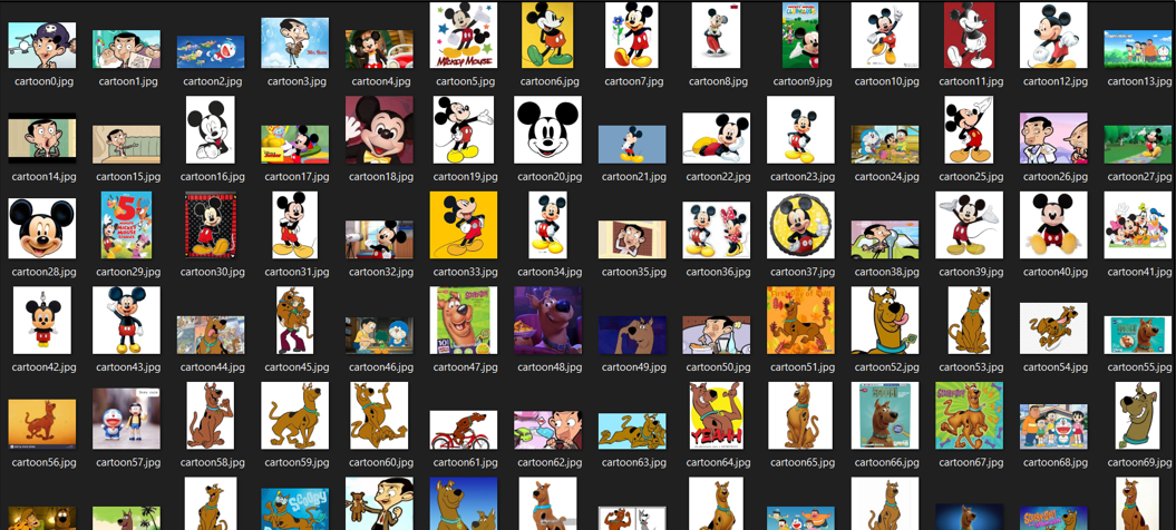
Always remember; if you feed garbage in, you get garbage out. To obtain the best results, make sure you collect enough images for the model to learn the features from it.

Once you have collected enough data, let’s proceed to the next step.

Label the dataset

To label the objects in the dataset, we’ll need an annotation/labeling tool. A lot of annotation tools are available to do so, such as LabelImg, Intel OpenVINO CVAT, VGG Image Annotator, etc. Although all these are the best annotation tools in the business, I find LabelImg easier to use. Hence, I go with it. Feel free to choose any annotation tool of your choice or simply follow this article as it is.

Below is an example of how an annotated image looks like – A bounding box around the region of interest (the object) and its label name.

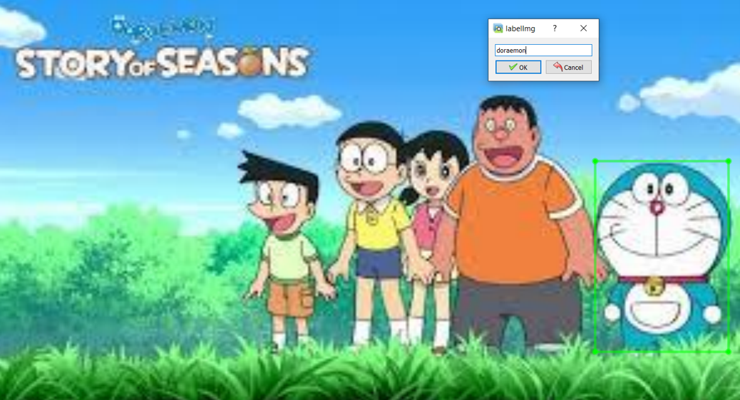
Image Annotation [Image source: Snapshot of data annotation on LabelImg on my local machine]

For every image annotated, a corresponding XML file will be generated which contains metadata such as, the coordinates of the bounding box, the class names, image name, image path, etc. This information will be required while training the model. We will see that part later as we move ahead.

Here is an example of how the annotation XML file looks like.

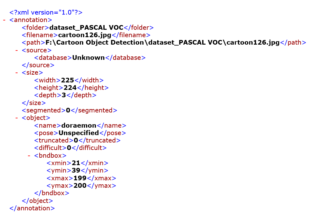
Annotation XML file [Image source: Screenshot of the XML file on my local machine]

Okay, once you have annotated all the images correctly, split the dataset into train and test sets in the following manner of the directory structure:

Upload dataset on Google Drive

Sign in to your Google account and upload the zipped dataset on your Google Drive. We will fetch this dataset during model training.

Make sure that the uploading of the dataset is not interrupted due to a network issue and is completely uploaded.

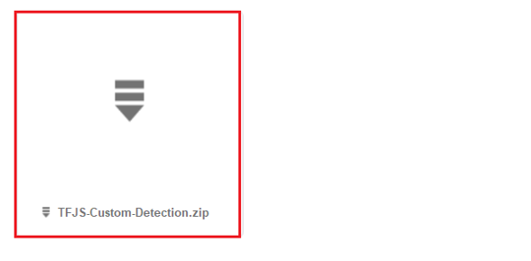
Dataset on Google Drive [Image source: Snapshot of the dataset uploaded on my Google Drive account]

Clone the following repository on your local machine

https://github.com/NSTiwari/TensorFlow.js-Custom-Object-Detection

This repository contains a Colab notebook named:
Custom_Object_Detection_using_TensorFlow_js.pynb.

Open Google Colab and upload this Colab notebook there. Now, we are going to start the actual training of our object detection model.

We are using Google Colab so that you do not need to install TensorFlow and other libraries on your local machine and thus we avoid the unnecessary hassle of manual installation of libraries, which may possibly go wrong if not done properly.

Configure Google Colab

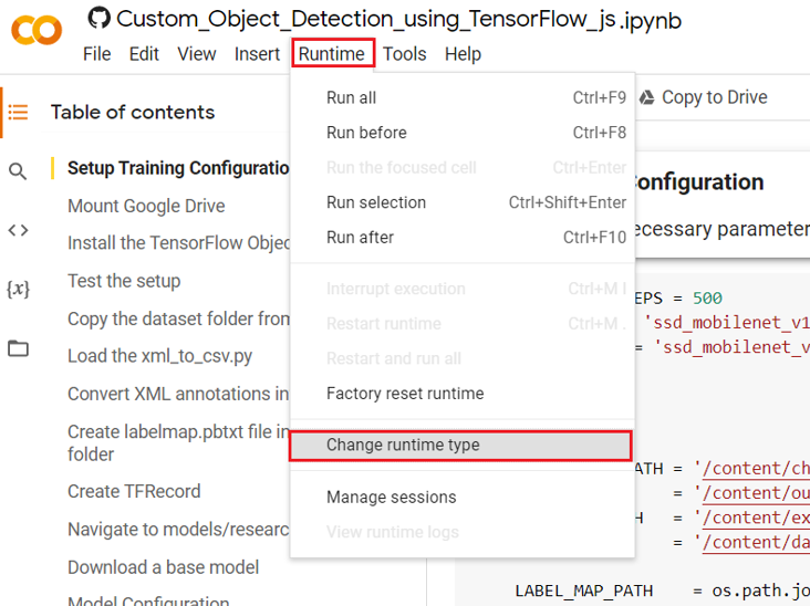
Once you have uploaded the notebook on Google Colab, check if the runtime type is set to ‘GPU’ or not. To do so, click on Runtime –> Change runtime type.

 

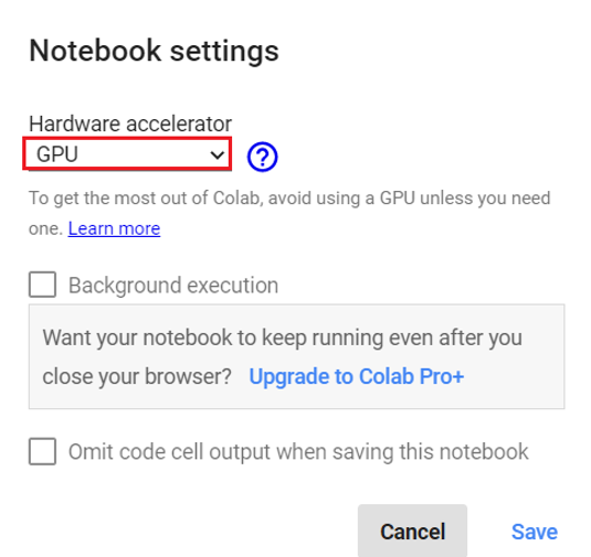
In the notebook settings, if the hardware accelerator is set to ‘GPU’, as shown below, you are good to go.

If you are done with all the above five steps successfully, let the actual game begin – Model Training.

Model Training

Configure all the necessary parameters for training.

NUM_TRAIN_STEPS = 500
MODEL_TYPE = 'ssd_mobilenet_v1_quantized_300x300_coco14_sync_2018_07_18'
CONFIG_TYPE = 'ssd_mobilenet_v1_quantized_300x300_coco14_sync'
import os
CHECKPOINT_PATH = '/content/checkpoint'
OUTPUT_PATH     = '/content/output'
EXPORTED_PATH   = '/content/exported'
DATA_PATH       = '/content/data'
LABEL_MAP_PATH    = os.path.join(DATA_PATH, 'labelmap.pbtxt')
TRAIN_RECORD_PATH = os.path.join(DATA_PATH, 'train.record')
VAL_RECORD_PATH   = os.path.join(DATA_PATH, 'val.record')

Mount Google Drive:
To access the dataset you stored on Google Drive in Step 3.

from google.colab import drive
drive.mount('/content/drive')

Install the TensorFlow Object Detection API:
Install and setup TensorFlow Object Detection API, Protobuf and other necessary dependencies.

Dependencies:
Most of the dependencies required come preloaded in Google Colab. The only additional package we need to install is TensorFlow.js, which is used for converting our trained model to a model that is compatible for the web.

Protocol Buffers:

Environment:
To use the object detection API, we need to add it to our PYTHONPATH along with slim which contains code for training and evaluating several widely used Convolutional Neural Network (CNN) image classification models.

%tensorflow_version 1.x

import os

import pathlib




# Clone the tensorflow models repository if it doesn't already exist

if "models" in pathlib.Path.cwd().parts:

  while "models" in pathlib.Path.cwd().parts:

    os.chdir('..')

elif not pathlib.Path('models').exists():

  !git clone --depth 1 https://github.com/cloud-annotations/models




!pip install cloud-annotations==0.0.4

!pip install tf_slim

!pip install lvis

!pip install --no-deps tensorflowjs==1.4.0




%cd /content/models/research

!protoc object_detection/protos/*.proto --python_out=.




pwd = os.getcwd()

os.environ['PYTHONPATH'] += f':{pwd}:{pwd}/slim'

Test the setup:

Run the model builder test to verify if everything is setup successfully.

!python object_detection/builders/model_builder_tf1_test.py

Copy the dataset folder from Google Drive:

Get the dataset of images and annotations saved on your Drive.

!unzip /content/drive/MyDrive/TFJS-Custom-Detection -d /content/
%cd /content/
%mkdir data

Load the xml_to_csv.py file:

!wget https://raw.githubusercontent.com/NSTiwari/TensorFlow.js-Custom-Object-Detection/master/xml_to_csv.py -P /content/TFJS-Custom-Detection/

Convert the XML annotations into a CSV file:

All the PascalVOC labels are converted into a CSV file for training and testing data.

%cd /content/
!python TFJS-Custom-Detection/xml_to_csv.py

Create labelmap.pbtxt file insde the data folder:

Consider the following example:

item {
  name: "doraemon"
  id: 1
}
item {
  name: "mickey_mouse"
  id: 2
}
item {
  name: "mr_bean"
  id: 3
}
item {
name: "mcqueen"
id: 4
}
item {
name: "scooby_doo"
id: 5
}

Create TFRecord:

Download the generate_tf_record.py file.

!wget https://raw.githubusercontent.com/NSTiwari/TensorFlow.js-Custom-Object-Detection/master/generate_tf_records.py -P /content/

!python generate_tf_records.py -l /content/data/labelmap.pbtxt -o data/train.record -i TFJS-Custom-Detection/images -csv TFJS-Custom-Detection/train_labels.csv
!python generate_tf_records.py -l /content/data/labelmap.pbtxt -o data/val.record -i TFJS-Custom-Detection/images -csv TFJS-Custom-Detection/val_labels.csv

Navigate to models/research directory:

%cd /content/models/research

Download a base model:

Training a model from scratch can take a lot of computation time. Instead, we choose to apply Transfer Learning on a pre-trained model. Transfer Learning helps to decrease computations and time, of course, to a great extent. The base model we’ll be using is the MobileNet model which is very fast.

import os
import tarfile

import six.moves.urllib as urllib

download_base = 'http://download.tensorflow.org/models/object_detection/'
model = MODEL_TYPE + '.tar.gz'
tmp = '/content/checkpoint.tar.gz'

if not (os.path.exists(CHECKPOINT_PATH)):
  # Download the checkpoint
  opener = urllib.request.URLopener()
  opener.retrieve(download_base + model, tmp)

  # Extract all the `model.ckpt` files.
  with tarfile.open(tmp) as tar:
    for member in tar.getmembers():
      member.name = os.path.basename(member.name)

      if 'model.ckpt' in member.name:
        tar.extract(member, path=CHECKPOINT_PATH)

  os.remove(tmp)

Model Configuration:

Before the training begins, we need to configure the training pipeline by specifying the paths for labelmap, TFRecord and checkpoint. The default batch size is 128 which also needs to be changed as it is too large to be handled by Colab.

import re

from google.protobuf import text_format

from object_detection.utils import config_util
from object_detection.utils import label_map_util

pipeline_skeleton = '/content/models/research/object_detection/samples/configs/' + CONFIG_TYPE + '.config'
configs = config_util.get_configs_from_pipeline_file(pipeline_skeleton)

label_map = label_map_util.get_label_map_dict(LABEL_MAP_PATH)
num_classes = len(label_map.keys())
meta_arch = configs["model"].WhichOneof("model")

override_dict = {
  'model.{}.num_classes'.format(meta_arch): num_classes,
  'train_config.batch_size': 24,
  'train_input_path': TRAIN_RECORD_PATH,
  'eval_input_path': VAL_RECORD_PATH,
  'train_config.fine_tune_checkpoint': os.path.join(CHECKPOINT_PATH, 'model.ckpt'),
  'label_map_path': LABEL_MAP_PATH
}


configs = config_util.merge_external_params_with_configs(configs, kwargs_dict=override_dict)
pipeline_config = config_util.create_pipeline_proto_from_configs(configs)
config_util.save_pipeline_config(pipeline_config, DATA_PATH)

Start Training:

Run the cell below to start training the model. Training is invoked by calling the model_main script and passing the following arguments to it.

• • The location of the pipeline.config we created.
• • Where we want to save the model.
• • How many steps we want to train the model (the longer you train, the more potential there is to learn).
• • The number of evaluation steps (or how often to test the model) gives us an idea of how well the model is doing.

!rm -rf $OUTPUT_PATH
!python -m object_detection.model_main 
    --pipeline_config_path=$DATA_PATH/pipeline.config 
    --model_dir=$OUTPUT_PATH 
    --num_train_steps=$NUM_TRAIN_STEPS 
    --num_eval_steps=100

Export Inference Graph:

Checkpoints are generated after every 500 training steps. Each checkpoint is a snapshot of your model at that point in training. If for some reason the training crashes due to network or power failure, then you can continue the training from the last checkpoint instead of starting it all over.

import os
import re

regex = re.compile(r"model.ckpt-([0-9]+).index")
numbers = [int(regex.search(f).group(1)) for f in os.listdir(OUTPUT_PATH) if regex.search(f)]
TRAINED_CHECKPOINT_PREFIX = os.path.join(OUTPUT_PATH, 'model.ckpt-{}'.format(max(numbers)))

print(f'Using {TRAINED_CHECKPOINT_PREFIX}')

!rm -rf $EXPORTED_PATH
!python -m object_detection.export_inference_graph 
  --pipeline_config_path=$DATA_PATH/pipeline.config 
  --trained_checkpoint_prefix=$TRAINED_CHECKPOINT_PREFIX 
  --output_directory=$EXPORTED_PATH

Testing the model:

Now, let’s test the model on some images. Remember that the model was trained only for 500 steps. So, the accuracy might not be that great. Run the cell below to test the model for yourself and find out how well the model was trained.

Note: Sometimes, this command doesn’t run, so, re-run it. Also, try training the model for 5,000 steps and see how the accuracy changes.

from IPython.display import display, Javascript, Image
from google.colab.output import eval_js
from base64 import b64decode
import tensorflow as tf

# Use javascipt to take a photo.
def take_photo(filename, quality=0.8):
  js = Javascript('''
    async function takePhoto(quality) {
      const div = document.createElement('div');
      const capture = document.createElement('button');
      capture.textContent = 'Capture';
      div.appendChild(capture);

const video = document.createElement('video');
      video.style.display = 'block';
      const stream = await navigator.mediaDevices.getUserMedia({video: true});

document.body.appendChild(div);
      div.appendChild(video);
      video.srcObject = stream;
      await video.play();

// Resize the output to fit the video element.
      google.colab.output.setIframeHeight(document.documentElement.scrollHeight, true);

// Wait for Capture to be clicked.
      await new Promise((resolve) => capture.onclick = resolve);

const canvas = document.createElement('canvas');
      canvas.width = video.videoWidth;
      canvas.height = video.videoHeight;
      canvas.getContext('2d').drawImage(video, 0, 0);
      stream.getVideoTracks()[0].stop();
      div.remove();
      return canvas.toDataURL('image/jpeg', quality);

    }
    ''')
  display(js)
  data = eval_js('takePhoto({})'.format(quality))
  binary = b64decode(data.split(',')[1])
  with open(filename, 'wb') as f:
    f.write(binary)
  return filename

try:
  take_photo('/content/photo.jpg')
except Exception as err:
  # Errors will be thrown if the user does not have a webcam or if they do not
  # grant the page permission to access it.
  print(str(err))

# Use the captured photo to make predictions
%matplotlib inline

import os
import numpy as np
from matplotlib import pyplot as plt
from PIL import Image as PImage
from object_detection.utils import visualization_utils as vis_util
from object_detection.utils import label_map_util

# Load the labels
category_index = label_map_util.create_category_index_from_labelmap(LABEL_MAP_PATH, use_display_name=True)
# Load the model
path_to_frozen_graph = os.path.join(EXPORTED_PATH, 'frozen_inference_graph.pb')
detection_graph = tf.Graph()
with detection_graph.as_default():
  od_graph_def = tf.GraphDef()
  with tf.gfile.GFile(path_to_frozen_graph, 'rb') as fid:
    serialized_graph = fid.read()
    od_graph_def.ParseFromString(serialized_graph)
    tf.import_graph_def(od_graph_def, name='')
with detection_graph.as_default():
  with tf.Session(graph=detection_graph) as sess:
    # Definite input and output Tensors for detection_graph
    image_tensor = detection_graph.get_tensor_by_name('image_tensor:0')
    # Each box represents a part of the image where a particular object was detected.
    detection_boxes = detection_graph.get_tensor_by_name('detection_boxes:0')
    # Each score represent how level of confidence for each of the objects.
    # Score is shown on the result image, together with the class label.
    detection_scores = detection_graph.get_tensor_by_name('detection_scores:0')
    detection_classes = detection_graph.get_tensor_by_name('detection_classes:0')
    num_detections = detection_graph.get_tensor_by_name('num_detections:0')
    image = PImage.open('/content/photo.jpg')
    # the array based representation of the image will be used later in order to prepare the
    # result image with boxes and labels on it.
    (im_width, im_height) = image.size
    image_np = np.array(image.getdata()).reshape((im_height, im_width, 3)).astype(np.uint8)
    # Expand dimensions since the model expects images to have shape: [1, None, None, 3]
    image_np_expanded = np.expand_dims(image_np, axis=0)
    # Actual detection.
    (boxes, scores, classes, num) = sess.run(
        [detection_boxes, detection_scores, detection_classes, num_detections],
        feed_dict={image_tensor: image_np_expanded})
    # Visualization of the results of a detection.
    vis_util.visualize_boxes_and_labels_on_image_array(
        image_np,
        np.squeeze(boxes),
        np.squeeze(classes).astype(np.int32),
        np.squeeze(scores),
        category_index,
        use_normalized_coordinates=True,
        line_thickness=8)
    plt.figure(figsize=(12, 8))
    plt.imshow(image_np)

 

Converting the model into TFJS:

The model we exported works well with Python. However, to deploy it on the web browser, we need to convert it into TensorFlow.js so that it becomes compatible to be run directly on the browser

Also, the model only detects objects as the IDs specified in the label_map.pbtxt. Therefore, we also need to create a JSON list of all of our labels that can be mapped to the ID.

!tensorflowjs_converter 
  --input_format=tf_frozen_model 
  --output_format=tfjs_graph_model 
  --output_node_names='Postprocessor/ExpandDims_1,Postprocessor/Slice' 
  --quantization_bytes=1 
  --skip_op_check 
  $EXPORTED_PATH/frozen_inference_graph.pb 
  /content/model_web

import json

from object_detection.utils.label_map_util import get_label_map_dict

label_map = get_label_map_dict(LABEL_MAP_PATH)
label_array = [k for k in sorted(label_map, key=label_map.get)]

with open(os.path.join('/content/model_web', 'labels.json'), 'w') as f:
  json.dump(label_array, f)

!cd /content/model_web && zip -r /content/model_web.zip *

Download the model:
The TFJS model is now ready to be downloaded.

Note: Sometimes, this command doesn’t run or it will throw an error. Just try running it again.

You can also download the model by right-clicking on the model_web.zip file in the left sidebar file inspector.

from google.colab import files
files.download('/content/model_web.zip')

If you have reached here without a hassle, congratulations, you have successfully trained the model.

Deploy the model on a web application using TensorFlow.js.

Once the TFJS model is downloaded, copy the model_web folder inside the TensorFlow.js-Custom-Object-Detection/React_Web_App/public directory.

Now, run the following commands:

cd TensorFlow.js-Custom-Object-Detection/React_Web_App

npm install

npm start

Now, finally open localhost:3000 on your web browser and test the model for yourself.

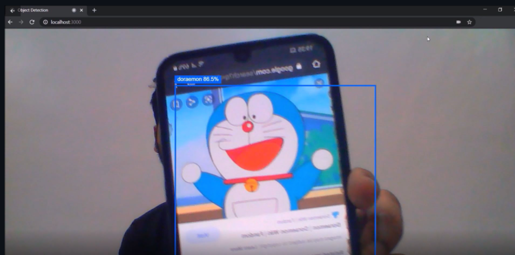
The object Detection output of the TF.js model [Image source: Snapshot of the TF.js model deployed on a React app on my local machine]

So, congratulations on creating an end-to-end custom object detection model using TensorFlow and deploying it on a web application using TensorFlow.js.

If you liked this article and would want to talk more about this, feel free to connect with me on LinkedIn