This article was published as a part of the Data Science Blogathon.
Introduction
As we all know, OpenCV is a free open source library used for computer vision and image operations. OpenCV is written in C++ and has thousands of optimized algorithms and functions for various image operations. A lot of real-life operations can be solved using OpenCV. These are video and image analysis, real-time computer vision, object detection, footage analysis, etc. Many companies, researchers and developers have contributed to the creation of OpenCV. Using OpenCV is straightforward, and OpenCV is equipped with many tools and functions. Let us use OpenCV to perform interesting image operations and look at the results.
Morphological Transformations
Morphological Transformations are image processing methods that transform images based on shapes. This process is helpful in the representation and depiction of regional shape. These transformations use a structuring element applied to the input image, and the output image is generated. Morphological operations have various uses, including removing noise from images, locating intensity bumps and holes in an image and joining disparate elements in images. There are two main types of Morphological Transformations.
They are Erosion and Dilation.
Erosion
Erosion is the morphological operation that is performed to reduce the size of the foreground object. The boundary of the foreign object is slowly eroded. Erosion has many applications in image editing and transformations, and erosion shrinks the image pixels. Pixels on object boundaries are also removed. Implementation of erosion is straightforward in Python and can be implemented with the help of a kernel.
Let us get started with the code in Python to implement erosion.
First, we import Open CV and Numpy.
import cv2
import numpy as np
Now we read the image.
image = cv2.imread("image1.jpg")
The image:
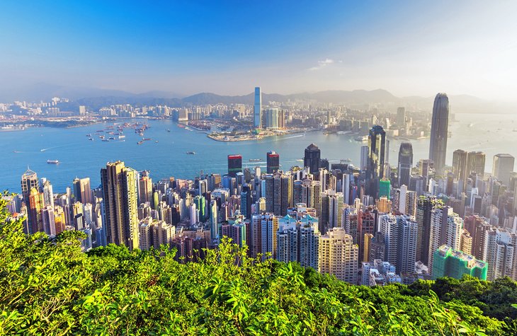
( Image Source: https://www.planetware.com/world/top-cities-in-the-world-to-visit-eng-1-39.htm )
We create a kernel needed to perform the erosion operation and implement it using an inbuilt OpenCV function.
# Creating kernel
kernel = np.ones((5, 5), np.uint8)
# Using cv2.erode() method
image_erode = cv2.erode(image, kernel)
Now, we save the file and have a look.
filename = 'image_erode1.jpg'
# Using cv2.imwrite() method
# Saving the image
cv2.imwrite(filename, image_erode)
The Image:
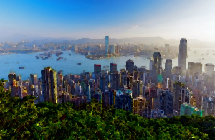
As we can see, the image is now eroded, sharpness and edges have reduced, and the image is blurred. Erosion can be used to hide or remove certain parts of an image or to hide information from images.
Let us try a different type of erosion.
kernel2 = np.ones((3, 3), np.uint8)
image_erode2 = cv2.erode(image, kernel2, cv2.BORDER_REFLECT)
Now, we save the image file.
filename = 'image_erode2.jpg'
# Using cv2.imwrite() method
# Saving the image
cv2.imwrite(filename, image_erode2)
The Image:
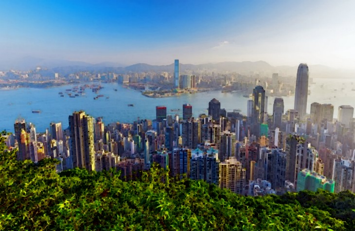
Now, let us see what Dilation is all about.
Dilation
Dilating the opposite process of erosion. In the case of Dilation, instead of shrinking, the foreground object is expanded. The things develop near the boundary, and an expanded object is formed. Bright regions in an image tend to “glow up” after Dilation, which usually results in an enhanced image. For this reason, Dilation is used in Image correction and enhancement.
Let us implement Dilation using Python code.
kernel3 = np.ones((5,5), np.uint8)
image_dilation = cv2.dilate(image, kernel, iterations=1)
Now, we save the image.
filename = 'image_dilation.jpg'
# Using cv2.imwrite() method
# Saving the image
cv2.imwrite(filename, image_dilation)
The Image:

As we can see, the image is now brighter and has more intensity.
Creating a Border
Adding a border to images is very simple, and our phone gallery app or editing app can do it very quickly. But, now let us create borders to our image using Python.
# Using cv2.copyMakeBorder() method
image_border1 = cv2.copyMakeBorder(image, 25, 25, 10, 10, cv2.BORDER_CONSTANT, None, value = 0)
Now, let us save the image.
filename = 'image_border1.jpg'
# Using cv2.imwrite() method
# Saving the image
cv2.imwrite(filename, image_border1)
The Image:
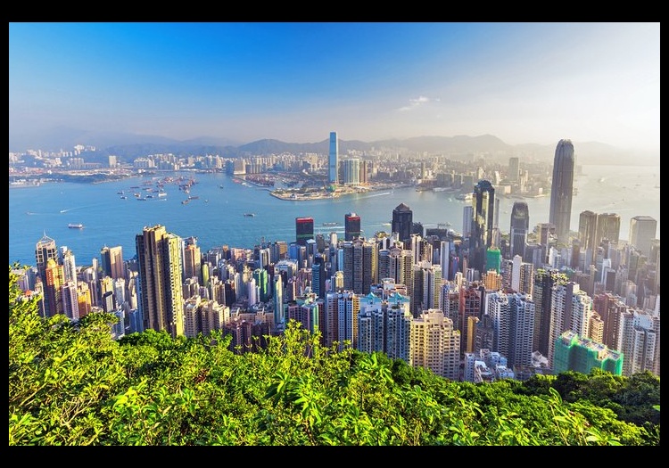
Here, we added a simple black border to the image. Now, let us try some mirrored borders.
#making a mirrored border
image_border2 = cv2.copyMakeBorder(image, 250, 250, 250, 250, cv2.BORDER_REFLECT)
Now, we save the image.
filename = 'image_border2.jpg'
# Using cv2.imwrite() method
# Saving the image
cv2.imwrite(filename, image_border2)
The Image:
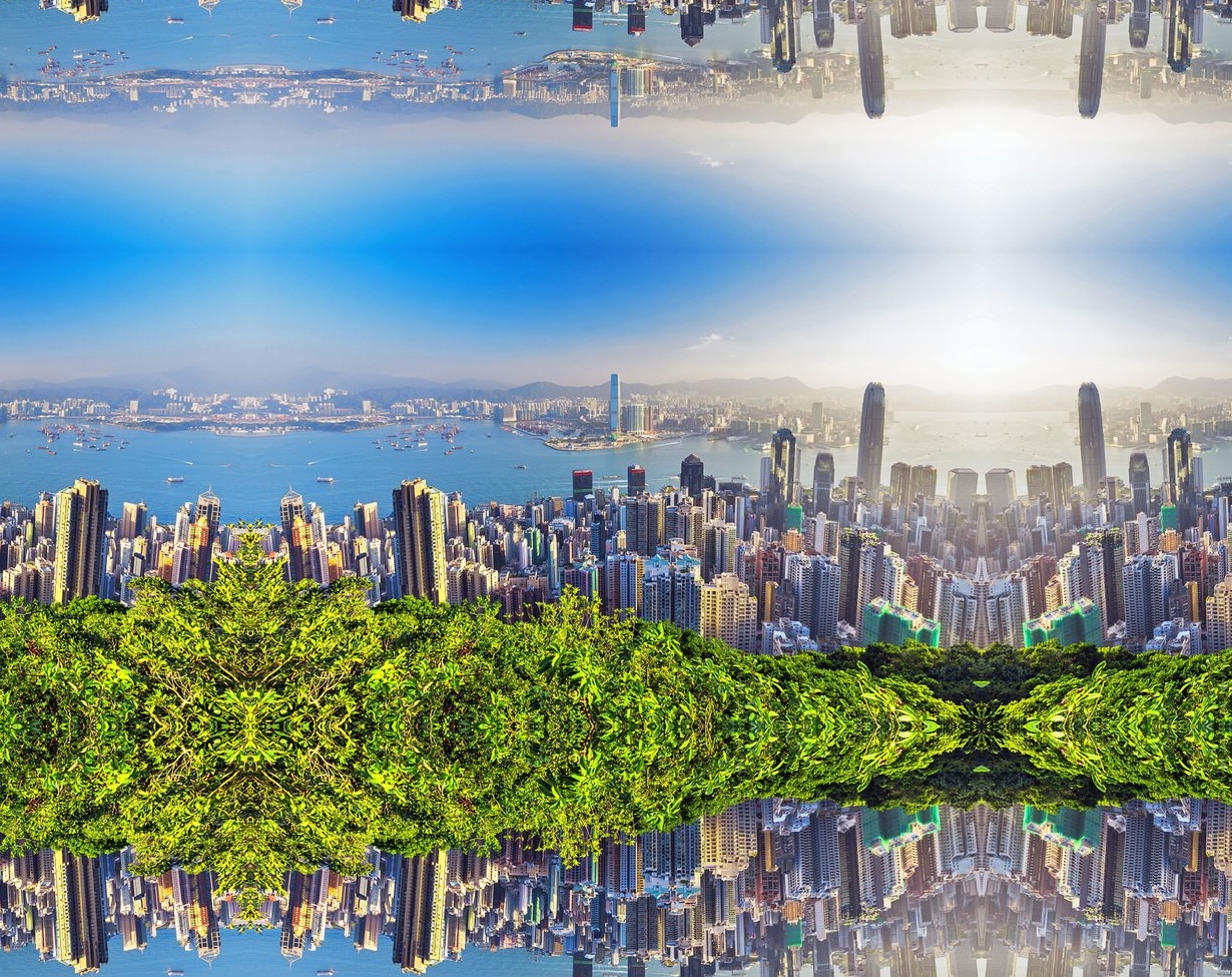
This is interesting, and it looks like something out of Dr Strange’s Mirror Dimension.
Let us try something else.
#making a mirrored border
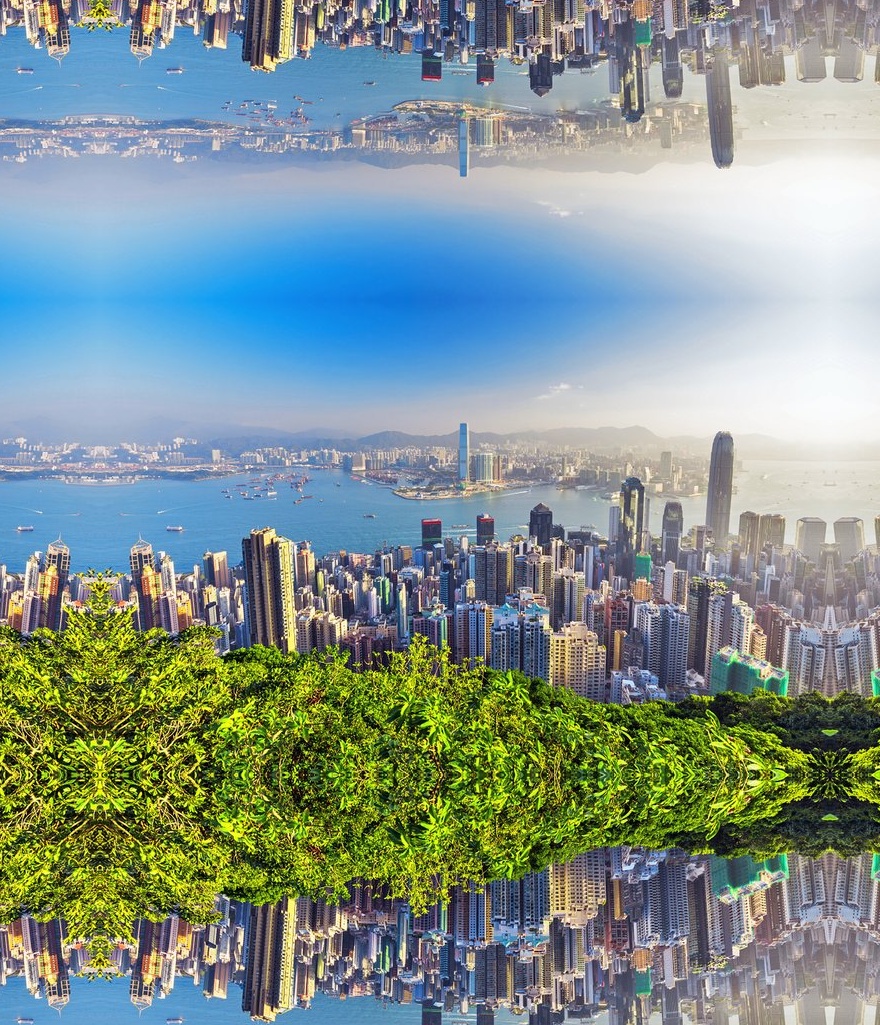
image_border3 = cv2.copyMakeBorder(image, 300, 250, 100, 50, cv2.BORDER_REFLECT)
Now, we save the image.
filename = 'image_border3.jpg'
# Using cv2.imwrite() method
# Saving the image
cv2.imwrite(filename, image_border3)
The Image:
Intensity Transformation
Often, images are subject to intensity transformation due to various reasons. These are done in the spatial domain, direct, on the image pixels. Operations like Image Thresholding and Contrast Manipulation are done using Intensity transformations.
Log Transformation
Logarithmic Transformation is an Intensity Transformation operation where the pixel values in an Image are replaced with their logarithmic value. Logarithmic transformation is used to brighten images or enhance the image as it expands darker pixels of an image more than higher pixel values.
Let us implement log transformation.
# Apply log transform.
c = 255/(np.log(1 + np.max(image)))
log_transformed = c * np.log(1 + image)
# Specify the data type.
log_transformed = np.array(log_transformed, dtype = np.uint8)
Now, we save the image.
cv2.imwrite('log_transformed.jpg', log_transformed)
The Image:
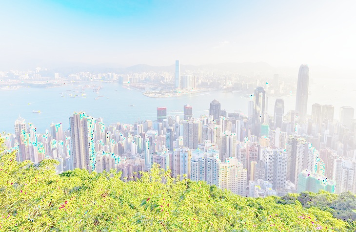
The image is made very bright.
Linear Transformation
We shall be applying a piecewise linear transformation to the images. This transformation is also done on the spatial domain. This method is used to modify images for a specific purpose. It is known as piecewise linear transformation as only a part of it is linear. The most commonly used piecewise Linear transformation is contrasted stretching.
Often, the resultant image has low contrast if images are clicked under low light and have bad surrounding illumination. Contrast stretching increases the range of intensity levels in an image, and the contrast stretching function increases monotonically so that the order of intensity of pixels is preserved.
Now, let us implement contrast stretching.
def pixelVal(pix, r1, s1, r2, s2):
    if (0 <= pix and pix <= r1):
        return (s1 / r1)*pix
    elif (r1 < pix and pix <= r2):
        return ((s2 - s1)/(r2 - r1)) * (pix - r1) + s1
    else:
        return ((255 - s2)/(255 - r2)) * (pix - r2) + s2
# Define parameters.
r1 = 70
s1 = 0
r2 = 140
s2 = 255
# Vectorize the function to apply it to each value in the Numpy array.
pixelVal_vec = np.vectorize(pixelVal)
# Apply contrast stretching.
contrast_stretch = pixelVal_vec(image, r1, s1, r2, s2)
# Save edited image.
cv2.imwrite('contrast_stretch.jpg', contrast_stretch)
The Image:
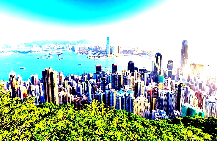
Here, the image is improved, and more contrast can be observed.
Denoising Colour Images
Denoising a signal or an image means removing the unnecessary signals and information to get the useful one. In the case of images, denoising is done to remove unwanted noise and analyze and process images better.
Let us denoise a colour image in Python.
denoised_image = cv2.fastNlMeansDenoisingColored(image, None, 15, 8, 8, 15)
Now, we save the image.
# Save edited image.
cv2.imwrite('denoised_image.jpg', denoised_image)
The Image:
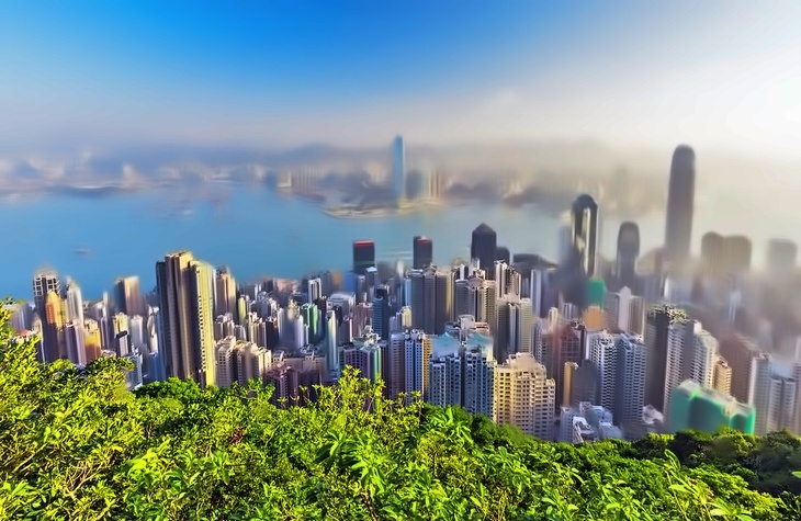
We can see a lot of wanted stuff like the background and the sky has been removed.
Analyze an image using Histogram
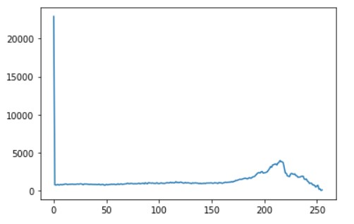
Histograms are an essential visual in any form of analysis. The Histogram of an image is an exciting way to understand the global description, and Histogram can be used to perform quantitative analysis on an image. An image histogram represents a grey level’s occurrence in an image.
We can understand the pixel intensity distribution of a digital image using a Histogram, and we can also use a Histogram to understand the dominant colours.
Let us plot a Histogram.
from matplotlib import pyplot as plt
histr = cv2.calcHist([image],[0],None,[256],[0,256])
plt.plot(histr)
Output:
# alternative way to find histogram of an image
plt.hist(image.ravel(),256,[0,256])
plt.show()
Output:
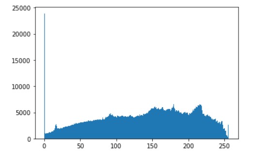
The plot shows the number of pixels on the image in the colour range of 0 to 255. We can see that there is a good distribution of all types of colours.
Now, let us convert the image to black and white and generate the Histogram.
grey_image = cv2.cvtColor(image, cv2.COLOR_BGR2GRAY)
histogram = cv2.calcHist([grey_image], [0], None, [256], [0, 256])
plt.plot(histogram, color='k')
Output:
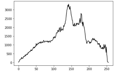
There is a big difference between this distribution and the previous one. Thi and this is mainly because the image was converted to greyscale and then analyzed.
Now, we perform the colour histogram.
for i, col in enumerate(['b', 'g', 'r']):
    hist = cv2.calcHist([image], [i], None, [256], [0, 256])
    plt.plot(hist, color = col)
    plt.xlim([0, 256])
plt.show()
Output:
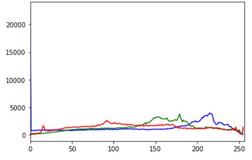
We can see that the number of pixels for blue and green is way higher than those for red. This is evident as there are a lot of blue and green areas in the image.
So we can see that plotting an image histogram is a great way to understand the image intensity distribution.
We had a look at some exciting applications of Computer Vision.
Check the code here: Link
Did you like my article? Please share in the comments below.
Connect with me on Linkedin.
My other articles on Analytics Vidhya: Link.
Thank You.


