The Guide to Data Analysis with DuckDB

This article was published as a part of the Data Science Blogathon.

Reach the next level in your data analysis career by adding DuckDB into your data stack. The guide will help you to understand Python API and various ways to read CSV files with SQL script.

The life of a data analyst revolves around loading data through SQL serve, analyzing it using various Python packages, and finally creating the technical report. Sometimes these SQL queries can take a longer time to process as we are dealing with terabytes of data. In this fast-paced world, this strategy fails miserably and most analytics are moving away from traditional ways to doing data analytics. DuckDB solves all the issues, it is integrated with Python & R. It works similarly to SQLite and focuses on providing faster analytical queries.

In this guide, we are going to learn various ways of running DuckDB SQL queries and also learn about Deepnote integration.

DuckDB

DuckDB is a relational table-oriented database management system and supports SQL queries for producing analytical results. It also comes with various features that are useful for data analytics.

Fast Analytical Queries

DuckDB is designed to run faster analytical queries workloads. It runs on a columnar-vectorized query execution engine that runs a large batch of processes in one go. This makes it faster to run Online analytical processing (OLAP) as compared to traditional systems such as PostgreSQL which process each row sequentially.

Simple Operation

DuckDB adopts simplicity and embedded operation.

• Serverless database with no external dependencies
• Doesn’t import or copy data while processing queries
• Embedded within a host process
• high-speed data transfer

Feature-Rich

DuckDB allows users to run complex SQL queries smoothly. It also supports secondary indexing to provide fast queries time within the single-file database. DuckDB provides full integration for Python and R so that the queries could be executed within the same file.

Free & Open Source

DuckDB is free to use and the entire code is available on GitHub. It comes with an MIT license which means you can use it for commercial purposes.

Creating Database

DuckDB provides out of box experience for you to connect with a database or create a new one with a similar command duckdb.connect(,read_only=False) .

As you can see in the image below SampleDB files have been created in your directory.

import duckdb
conn = duckdb.connect(“SampleDB”,read_only=False)

OR

DuckDB also allows you to create an in-memory temporary database by using duckdb.connect(). The conn.execute() run all the queries requests in the database. In this example, we are going to create a temporary table called test_table which contains i as integer and j as a string. If you are familiar with SQL you won’t have a problem understanding query requests, but if you are new to SQL, I will suggest you look at this amazing cheat sheet.

conn = duckdb.connect()

# run arbitrary SQL commands
conn.execute(“CREATE TABLE test_table (i INTEGER, j STRING)”)

Inserting values

You can insert single or multiple values by using SQL commands. In this part, we are adding two values to test_table using execute.

conn.execute(“INSERT INTO test_table VALUES (1, ‘one’),(9,’nine’)”)

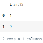
To check whether we have successfully added values we are going to run SQL to read all values of i. To display the result of queries in Pandas dataframe we will add .fetchdf() as shown below. Good Job, We have successfully added our filet two values.

conn.execute(“SELECT i from test_table “).fetchdf()

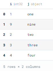
We can also use placeholders for parameters and then add an array to the test_table. If you are familiar with the Python framework, you will find this method easy to execute. We can also execute multiple values at once by using .executemany(). As you can see below how we have successfully added values into the test_table.

conn.execute(“INSERT INTO test_table VALUES (?, ?)”, [2, ‘two’])

conn.executemany(“INSERT INTO test_table VALUES (?, ?)”, [[3, ‘three’], [4, ‘four’]])

conn.execute(“SELECT * from test_table “).fetchdf()

Use .fetchnumpy() to display your results in form of a NumPy array. From this point this will get quite interesting as we will be learning various ways to execute complex SQL queries for data analysis

conn.execute(“SELECT * FROM test_table”).fetchnumpy()

{'i': array([1, 9, 2, 3, 4, 1, 9, 2, 3, 4, 1, 9, 2, 3, 4, 1, 9, 2, 3, 4, 1, 9,
        2, 3, 4, 1, 9, 2, 3, 4], dtype=int32),
 'j': array(['one', 'nine', 'two', 'three', 'four', 'one', 'nine', 'two',
        'three', 'four', 'one', 'nine', 'two', 'three', 'four', 'one',
        'nine', 'two', 'three', 'four', 'one', 'nine', 'two', 'three',
        'four', 'one', 'nine', 'two', 'three', 'four'], dtype=object)}

Pandas Data Frame and SQL

In this section, we are going to play around with Panda’s dataframe and learn various ways to read .csv files. First, we are going to create a simple Pandas dataframe using a dictionary and then we are going to add it to a new table called test_df.

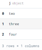
Using SQL script to find all the values of j where i is greater than one. The query results show three samples matching our conditions.

import pandas as pd

test_df = pd.DataFrame.from_dict({“i”:[1, 2, 3, 4], “j”:[“one”, “two”, “three”, “four”]})

conn.register(“test_df”, test_df)

conn.execute(“SELECT j FROM test_df WHERE i > 1”).fetchdf()

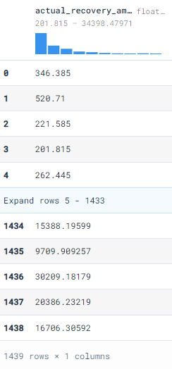
In the next step, we are going to import .csv to pandas data frame and then add it to the new table bank_df. The data set used in this example is from Kaggle under the GPL2 license. The results show the actual recovery amount where the age is greater than 27. As we can see that the complex queries are getting simple to execute.

df = pd.read_csv(“bank_data.csv”)

conn.register(“bank_df”, df)

conn.execute(“SELECT actual_recovery_amount FROM bank_df WHERE age > 27”).fetchdf()

Relations

Relation API uses programmatic queries to evaluate chains f relations commands. In short, you can run python functions on relations and display the results. The results contain an experienced Tree, results in columns, and results in a preview. If you are feeling confused right now then it’s ok because we are going to go deep into relations and how to use them to get analytical results.

Loading Relations

Creating relation from existing Pandas dataframe test_df using conn.from_df(test_df) . By printing, rel we can visualize the entire dataframe.

rel = conn.from_df(test_df)

rel

---------------------
-- Expression Tree --
---------------------
pandas_scan(140194817412592)

---------------------
-- Result Columns --
---------------------
- i (BIGINT)
- j (VARCHAR)

---------------------
-- Result Preview --
---------------------
i j
BIGINT VARCHAR
[ Rows: 4] 1 one
2 two
3 three
4 four

You can also use duckdb.df() it for similar results.

rel = duckdb.df(test_df)

Use conn.table to create a relation from the existing table. In our case, we are using test_table.

rel = conn.table(“test_table”)

rel

---------------------
-- Expression Tree --
---------------------
Scan Table [test_table]

---------------------
-- Result Preview --
---------------------
i j
INTEGER VARCHAR
[ Rows: 5] 1 one
9 nine
2 two
3 three
4 four

In order to create the relation directly from .csv file, use .from_csv_auto .

rel = duckdb.from_csv_auto(“bank_data.csv”)

rel

---------------------
-- Expression Tree --
---------------------
read_csv_auto(bank_data.csv)

---------------------
-- Result Columns  --
---------------------
- id (INTEGER)
- expected_recovery_amount (INTEGER)
- actual_recovery_amount (DOUBLE)
- recovery_strategy (VARCHAR)
- age (INTEGER)
- sex (VARCHAR)
---------------------
-- Result Preview  --
---------------------
id	expected_recovery_amount	actual_recovery_amount	recovery_strategy	age	sex	
INTEGER	INTEGER	DOUBLE	VARCHAR	INTEGER	VARCHAR	
[ Rows: 10]
2030	194	263.540000	Level 0 Recovery	19	Male	
1150	486	416.090000	Level 0 Recovery	25	Female	
380	527	429.350000	Level 0 Recovery	27	Male	
1838	536	296.990000	Level 0 Recovery	25	Male	
1995	541	346.385000	Level 0 Recovery	34	Male	
731	548	520.710000	Level 0 Recovery	35	Male	
221	549	221.585000	Level 0 Recovery	33	Male	
1932	560	373.720000	Level 0 Recovery	19	Female	
1828	562	201.865000	Level 0 Recovery	22	Female	
2001	565	504.885000	Level 0 Recovery	27	Male

Relational Information

Use rel.alias to check the name given to the relation. In our case it’s bank_data.csv.

rel.alias

'bank_data.csv'

We can change the current alias by using .set_alias . This might get useful for joining similar relations.

rel2 = rel.set_alias(‘bank_data’)

rel2.alias

'bank_data'

The type of our relations in Subquery_Relation.

rel.type

'SUBQUERY_RELATION'

To inspect the columns name of relation, just use .columns .

rel.columns

['id',
 'expected_recovery_amount',
 'actual_recovery_amount',
 'recovery_strategy',
 'age',
 'sex']

Use .types to inspect columns types.

rel.types

['INTEGER', 'INTEGER', 'DOUBLE', 'VARCHAR', 'INTEGER', 'VARCHAR']

Applying Python like functions (Single function)

Now comes the fun part. You can add any function with the relation and it will display augmented results. In our case, we have used rel.filter and it displays results of age greater than 18. It’s also displaying additional information about the expression tree, which can be quite useful if you have a long complex query to run.

rel.filter(‘age > 18’)

---------------------
-- Expression Tree --
---------------------
Filter [age>18]
  read_csv_auto(bank_data.csv)

---------------------
-- Result Columns  --
---------------------
- id (INTEGER)
- expected_recovery_amount (INTEGER)
- actual_recovery_amount (DOUBLE)
- recovery_strategy (VARCHAR)
- age (INTEGER)
- sex (VARCHAR)
---------------------
-- Result Preview  --
---------------------
id	expected_recovery_amount	actual_recovery_amount	recovery_strategy	age	sex	
INTEGER	INTEGER	DOUBLE	VARCHAR	INTEGER	VARCHAR	
[ Rows: 10]
2030	194	263.540000	Level 0 Recovery	19	Male	
1150	486	416.090000	Level 0 Recovery	25	Female	
380	527	429.350000	Level 0 Recovery	27	Male	
1838	536	296.990000	Level 0 Recovery	25	Male	
1995	541	346.385000	Level 0 Recovery	34	Male	
731	548	520.710000	Level 0 Recovery	35	Male	
221	549	221.585000	Level 0 Recovery	33	Male	
1932	560	373.720000	Level 0 Recovery	19	Female	
1828	562	201.865000	Level 0 Recovery	22	Female	
2001	565	504.885000	Level 0 Recovery	27	Male

Using .project will display mentioned columns and in our case is displaying id and age.

rel.project(‘id, age’)

---------------------
-- Expression Tree --
---------------------
Projection [id, age]
  read_csv_auto(bank_data.csv)

---------------------
-- Result Columns  --
---------------------
- id (INTEGER)
- age (INTEGER)

You can transform your columns values by adding a number or using any arithmetic function. In our case, it’s displaying age with +1.

rel.project(‘age + 1’)

---------------------
-- Expression Tree --
---------------------
Projection [age + 1]
  read_csv_auto(bank_data.csv)

---------------------
-- Result Columns  --
---------------------
- age + 1 (INTEGER)
---------------------
-- Result Preview  --
---------------------
age + 1	
INTEGER	
[ Rows: 10]
20	
26	
28	
26	
35	
36	
34	
20	
23	
28

Order is similar to SQL script ORDER .

rel.order(‘sex’)

The .limit shows top samples in a table. In our case, it will only display the top 2 values.

rel.limit(2)

Stacking all the functions in a chain

Just like in R, you can stack all of your functions to get the SQL output. In our case, it’s displaying the top two actual_recovery_amount, order by sex of the people with the age greater than 27. We are now realizing the full potential of the expression tree.

rel.filter(‘age > 27’).project(‘actual_recovery_amount’).order(‘sex’).limit(2)
---------------------
-- Expression Tree --
---------------------
Limit 2
  Order [sex DESC]
    Projection [actual_recovery_amount]
      Filter [age>27]
        read_csv_auto(bank_data.csv)

---------------------
-- Result Columns  --
---------------------
- actual_recovery_amount (DOUBLE)
---------------------
-- Result Preview  --
---------------------
actual_recovery_amount	
DOUBLE	
[ Rows: 2]
278.720000	
245.000000

Aggregate functions

The aggregate function can perform multiple group tasks. In this case, it’s summing all the actual recovery amount.

rel.aggregate(“sum(actual_recovery_amount)”)

---------------------
-- Result Preview  --
---------------------
sum(actual_recovery_amount)	
DOUBLE	
[ Rows: 1]
7529821.469511

The function below will display the sum of actual_recovery_amount per age group. This is super cool as we have reduced two functions into one.

rel.aggregate(“age, sum(actual_recovery_amount)”)

---------------------
-- Result Preview  --
---------------------
age	sum(actual_recovery_amount)	
INTEGER	DOUBLE	
[ Rows: 10]
19	52787.712089	
25	72769.342330	
27	67569.292950	
34	109902.427032	
35	115424.466724	
33	138755.807230	
22	46662.153746	
31	92225.534688	
18	39969.573274	
32	110627.466806

If you want to only show the sum of actual _recovery amount then add group by columns as a secondary input. In our case, it’s only showing the sum of actual recovery amounts per age.

rel.aggregate(“sum(actual_recovery_amount)”, “age”)

---------------------
-- Result Preview  --
---------------------
sum(actual_recovery_amount)	
DOUBLE	
[ Rows: 10]
52787.712089	
72769.342330	
67569.292950	
109902.427032	
115424.466724	
138755.807230	
46662.153746	
92225.534688	
39969.573274	
110627.466806

To display unique values use distinct()

rel.distinct()

---------------------
-- Result Preview  --
---------------------
id	expected_recovery_amount	actual_recovery_amount	recovery_strategy	age	sex	
INTEGER	INTEGER	DOUBLE	VARCHAR	INTEGER	VARCHAR	
[ Rows: 10]
2030	194	263.540000	Level 0 Recovery	19	Male	
1150	486	416.090000	Level 0 Recovery	25	Female	
380	527	429.350000	Level 0 Recovery	27	Male	
1838	536	296.990000	Level 0 Recovery	25	Male	
1995	541	346.385000	Level 0 Recovery	34	Male	
731	548	520.710000	Level 0 Recovery	35	Male	
221	549	221.585000	Level 0 Recovery	33	Male	
1932	560	373.720000	Level 0 Recovery	19	Female	
1828	562	201.865000	Level 0 Recovery	22	Female	
2001	565	504.885000	Level 0 Recovery	27	Male

Multi-relation operators

We can create UNION between two relations by using .union This combines the results of both relations.

rel.union(rel)
---------------------
-- Expression Tree --
---------------------
Union
  read_csv_auto(bank_data.csv)  read_csv_auto(bank_data.csv)

Joining two relations on id column. We have created rel2 and joined it to rel based on id.

rel2 = duckdb.df(df)

rel.join(rel2, ‘id’)

---------------------
-- Expression Tree --
---------------------
Join
  read_csv_auto(bank_data.csv)  pandas_scan(139890483423984)

To join similar relation we will be using alias() to change the alias and then joining them as shown below.

rel.set_alias(‘a’).join(rel.set_alias(‘b’), ‘a.id=b.id’)

 — — — — — — — — — — — — Expression Tree — — — — — — — — — — — — Join read_csv_auto(bank_data.csv) read_csv_auto(bank_data.csv)

DuckDB Functions with a DataFrame.

We can skip creating relations and dive right into filtering and sorting by using duckdb.(,). The examples show how you can create results using Pandas dataframe directly.

print(duckdb.filter(df, ‘age > 1’))

print(duckdb.project(df, ‘age +1’))

print(duckdb.order(df, ‘sex’))

print(duckdb.limit(df, 2))

Similarly, we can create a chain of functions and display the results as shown below.

duckdb.filter(df, ‘age > 1’).project(‘age + 1’).order(‘sex’).limit(2)

---------------------
-- Expression Tree --
---------------------
Limit 2
  Order [sex DESC]
    Projection [age + 1]
      Filter [age>1]
        pandas_scan(139890483423984)

---------------------
-- Result Columns  --
---------------------
- age + 1 (BIGINT)
---------------------
-- Result Preview  --
---------------------
age + 1	
BIGINT	
[ Rows: 2]
26	
20

Relation Query Results in DuckDB

To display the results of the relation use:

1. fetchone(): to display only the first row and you can repeat this command until you have cycled through all.
   
2. fetchall(): to display all the values from results.
3. fetchdf(): to display results in form of Pandas Dataframe.
4. fethnumpy(): to display results in form of a Numpy array.

res = rel.execute()

print(res.fetchone())
(2030, 194, 263.54, ‘Level 0 Recovery’, 19, ‘Male’)

print(res.fetchall())

[(1150, 486, 416.09, ‘Level 0 Recovery’, 25, ‘Female’), (380, 527, 429.35, ‘Level 0 Recovery’, 27, ‘Male’).....

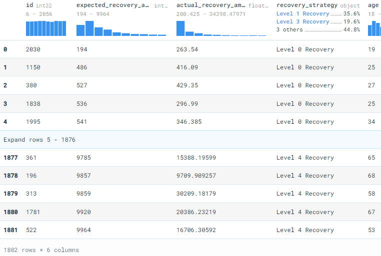
• We can also convert the results into Pandas dataframe by using rel.df() or rel.to_df() as shown below.

rel.to_df()

Tables and DuckDB

We can also create tables in relation by using .create

rel.create(“test_table2”)

In the next part, we are going to learn various ways to insert values into relation.

• Create a new table test_table3.
• Insert values using values() and insert_into()
• create a relation by using test_table3.
• Insert values into relation using simple .insert function.

As we can see we have successfully added a single value to the relation.

conn.execute(“CREATE TABLE test_table3 (i INTEGER, j STRING)”)

conn.values([5, ‘five’]).insert_into(“test_table3”)

rel_3 = conn.table(“test_table3”)

rel_3.insert([6,’six’])

rel_3

---------------------
-- Expression Tree --
---------------------
Scan Table [test_table3]

---------------------
-- Result Columns  --
---------------------
- i (INTEGER)
- j (VARCHAR)
---------------------
-- Result Preview  --
---------------------
i	j	
INTEGER	VARCHAR	
[ Rows: 2]
5	five	
6	six

DuckDB Query function

To run SQL queries directly you can use .query them with the relation. Then add the first input as the view name of the query and the second input as SQL script using the view name as shown below.

res = rel.query(‘my_name_for_rel’, ‘SELECT * FROM my_name_for_rel LIMIT 5’)

In order to see the results, let’s use fetchall() to display all 5 values.

res.fetchall()

[(2030, 194, 263.54, 'Level 0 Recovery', 19, 'Male'),
 (1150, 486, 416.09, 'Level 0 Recovery', 25, 'Female'),
 (380, 527, 429.35, 'Level 0 Recovery', 27, 'Male'),
 (1838, 536, 296.99, 'Level 0 Recovery', 25, 'Male'),
 (1995, 541, 346.385, 'Level 0 Recovery', 34, 'Male')]

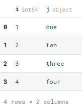
We can directly use .query() and run a query on the test_df table. The results show all four values from the table. The query function can perform all the functions on your table, dataframe, and even on .csv files.

res = duckdb.query(‘SELECT * FROM test_df’)

res.df()

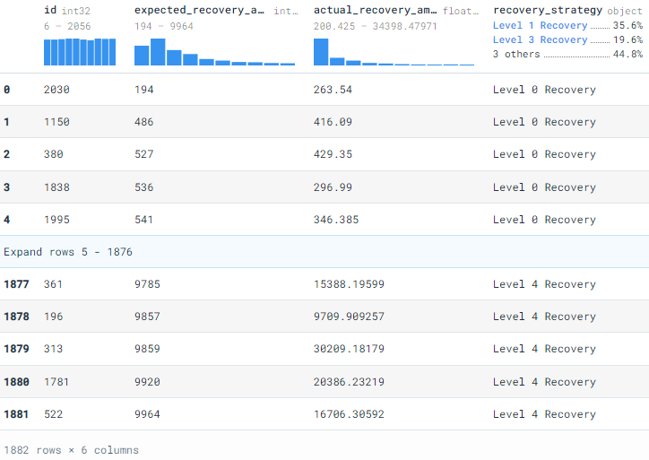
In order to run a query on .csv file, we will be using read_csv_auto() in SQL script. In our case, we are reading the entire data directly from a CSV file and displaying it in Pandas dataframe.

res = duckdb.query(“SELECT * FROM read_csv_auto(‘bank_data.csv’)”)

res.df()

Let’s run a complex script so that we can realize the full potential of DuckDB. The result below shows that more amount was recovered the expected from a female using the level 4 strategy. In my opinion, using SQL queries for data analysis is fast and fun, instead of loading your data into pandas and writing a bunch of code to get similar results.

res = duckdb.query(“SELECT sex, SUM(expected_recovery_amount) as Expected,
 SUM(actual_recovery_amount) as Actual 
 FROM ‘bank_data.csv’
 WHERE recovery_strategy LIKE ‘Level 4 Recovery’
 GROUP BY sex
 HAVING sex = ‘Female’”)
res.df()

Deepnote SQL Cell

Deepnote’s Dataframe SQL cell is using DuckDB on its backend, so if you want an easy way to use all the functions of DuckDB, I recommend you to use the Deepnote SQL cell. To run your SQL query first all add SQL cells from the block option.

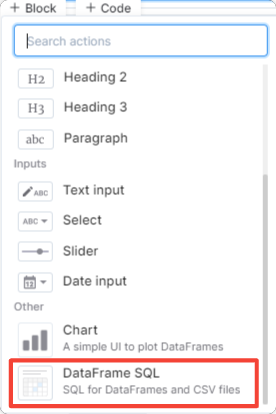
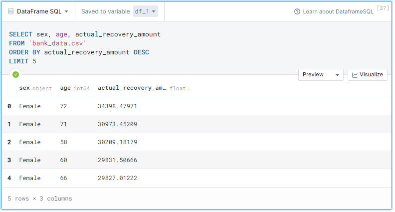
Try writing a simple SQL script. As we can see we are reading data directly from bank_data.csv and the results are stored in df_1 in form of Pandas DataFrame. I just love this feature, it’s even better than loading your data through Pandas.

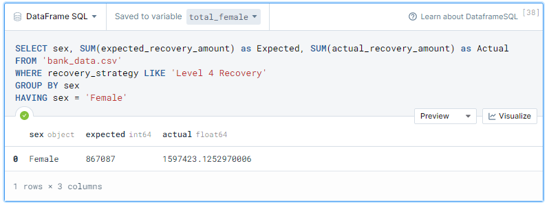
Let’s try a more complex SQL query on a CSV file. We will be displaying three columns sex, expected, and actual. Then, we will select values where recovery_strategy is ‘Level 4 Recovery’ and group by sex. Finally, we will only display female values.

Final thoughts on DuckDB

DuckDB can solve most of the issues present in traditional SQL databases. It is a serverless database management system with faster analytics queries and it’s completely integrated with Python and R. If you are going to deploy a data science or machine learning application I suggest you add DuckDB to your stack.

In this guide, we have learned various ways to create a database, add tables, and run queries. We have also learned about relations and we can use them to create complex functions. Finally, we have used various ways to directly interact with CSV files and ran multiple complex scripts. This guide includes all kinds of examples so if you get stuck in your project, you can come back and learn some tricks. In the end, I will always suggest you to learn the basics by practicing.

Learning Resources

• DuckDB: an embedded DB for data wrangling — DEV Community 👩‍💻👨‍💻
• SQL Tutorial (w3schools.com)
• DuckDB — SQL Introduction
• Intro to SQL Cells (deepnote.com)
• DataFrame SQL — Deepnote docs

About Author

Abid Ali Awan (@1abidaliawan) is a certified data scientist professional who loves building machine learning models and research on the latest AI technologies. Currently, testing AI Products at PEC-PITC, their work later gets approved for human trials, such as the Breast Cancer Classifier. His vision is to build an AI product that will identify students struggling with mental illness.

Data Science Portfolio Projects

• Deepnote
• GitHub
• DAGsHub
• Kaggle

The media shown in this article is not owned by Analytics Vidhya and are used at the Author’s discretion

Abid Ali Awan

I am a technology manager turned data scientist who loves building machine learning models and research on various AI technologies. My vision is to build an AI product that will help identify students who are struggling with mental illness.