Complete Guide to Anomaly Detection with AutoEncoders using Tensorflow

This article was published as a part of the Data Science Blogathon.

Data Preprocessing: Data preparation is critical in machine learning use cases. Data Compression is a big topic used in computer vision, computer networks, and many more. Data compression represents our input into a more miniature representation that we recreate to quality. This is a more miniature representation of what would be passed around, and when an original one is required, they will reconstruct it from a more miniature model.

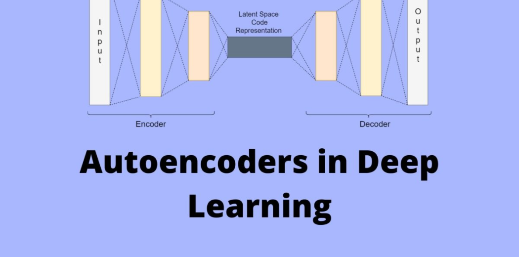
Table of Contents

1. Brief on AutoEncoders
2. why we need AutoEncoders?
3. Components of AutoEncoders
4. Properties of Autoencoders
5. Architecture of Autoencoders
6. Training of AutoEncoder
7. Applications of Autoencoders
8. Hands-on Implementation of Anomaly detection using AutoEncoders
9. End Notes

Introduction to AutoEncoders

AutoEncoders is a neural network that learns to copy its inputs to outputs. In simple words, AutoEncoders are used to learn the compressed representation of raw data. Autoencoders are based on unsupervised machine learning that applies the backpropagation technique and sets the target values equal to the inputs. It does here is simple dimensionality reduction, the same as the PCA algorithm. But the potential benefit is how they treat the non-linearity of data. It allows the Model to learn very powerful generalizations. And it can reconstruct the output back with lower significant loss of information than PCA. This is the advantage of AutoEncoder over PCA. Let us summarize Autoencoder in the below three key points.

• It is an unsupervised ML algorithm similar to PCA.
• It minimizes the same objective function as PCA.
• The neural network target output is its output.

Why do we need AutoEncoders?

Many have questions that if we already have PCA, why learn and use Autoencoder? Is it only because of its property to work on non-linear data? So the answer is No because apart from dealing with non-linear data, Autoencoder provides different applications from Computer vision to time series forecasting.

1. Non-linear Transformations – it can learn non-linear activation functions and multiple layers.
2. Convolutional layer – it doesn’t have to learn dense layers to use CNN or LSTM.
3. Higher Efficiency – More efficient in model parameters to learn several layers with an autoencoder rather than learn one huge transformation with PCA.
4. Multiple transformations – An autoencoder also gives a representation as to the output of each layer, and having multiple representations of different dimensions is always useful. An autoencoder lets you use pre-trained layers from another model to apply transfer learning to prime the encoder and decoder.

Components of AutoEncoders

Autoencoder is comprised of two parts named encoder and decoder. In some articles, you will also find three components, and the third component is a middleware between both known as code.

Encoders

It compresses the input into a latent space representation. The encoder layer encodes the input image as a compressed representation in a reduced dimension; now, the compressed image looks like the original image but not the original image.

Code

An encoder is mapping from input space into lower dimension latent space, also known as bottleneck layer(represented as z in architecture). At this stage, it is a lower-dimensional representation of data unsupervised. Code is the part that represents the compressed input fed to the decoder.

Decoder

The decoder decodes the encoded image back to the original image of the same dimension. The decoder takes the data from the lower latent space to the reconstruction phase, where the dimensionality of the output X bar is equal to output X. But if we look at it as Image compression, then there is lossless compression, but In the case of Autoencoders, there is lossy compression, so what happens is it compresses and uncompresses the input. When it uncompresses, it tries to reach close to input, but the output is not the same.

Properties of AutoEncoders

Let us look at the important properties passed by autoencoders.

1) Unsupervised – They do not need labels to train on.

2) data specific – They can only compress the data similar to what they have been trained on. for example, an autoencoder trained on the human face will not perform well on images of modern buildings. This improvises the difference between auto-encoder and mp3 kind of compression algorithm, which only holds assumptions about sound.

3) Lossy – Autoencoders are lossy, meaning the decompressed output will be degraded.

Architecture of AutoEncoder

Now let us understand the architecture of Autoencoder and have a deeper insight into the hidden layers. So in Autoencoder, we add a couple of layers between input and output, and the sizes of this layer are smaller than the input layer.

A critical part of the Autoencoder is the bottleneck. The bottleneck approach is a beautifully elegant approach to representation learning specifically for deciding which aspects of obs data are relevant information and which aspects can be thrown away. It describes by balancing two criteria.

1. The compactness of representation, measured as the compressibility number of bits needed to store compressibility.
2. Information the representation retains about some behaviorally relevant variables.

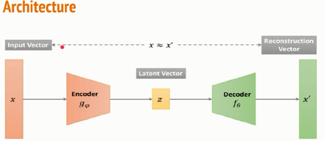
In this case, the difference between input representation and output representation is known as reconstruction error(error between input vector and output vector). One of the predominant use cases of the Autoencoder is anomaly detection. Think about cases like IoT devices, sensors in CPU, and memory devices which work very nicely as per functions. Still, when we collect their fault data, we have majority positive classes and significantly less percentage of minority class data, also known as imbalance data. Sometimes it is tough to label the data or expensive labelling the data, so we know the expected behaviour of data.

We pass Autoencoder with majority classes(normal data). The training objective is to minimize the reconstruction error, and the training objective is to minimize this. as training progresses, the model weights for the encoder and decoder are updated. The encoder is a downsampler, and the decoder is an upsampler. Encoder and decoder can be ANN, CNN, or LSTM neural network.

What AutoEncoder does? It learns the reconstruction function that works with normal data, and we can use this Model for anomaly detection. We get low reconstruction error for normal data and high for abnormal data(minority class).

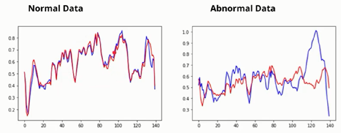
Reconstruction error is the difference between the red and blue lines, and this reconstruction error is undoubtedly high. So a model will not fit perfectly.

Training of AutoEncoders

There are four significant hyperparameters that we need to set before training them.

1) Code Size represents the number of nodes in the middle layer—the smaller size results in more compression.

2) Number of Layers – The Autoencoder can be as deep as we want to be.

3) Loss function – To update the weights, we must calculate the loss, which we need to minimize using optimizer and weight updation. Mainly mean squared error and binary cross-entropy. The input value is 0-1; then, we use cross-entropy. Otherwise, we use mean squared error.

4) Number of nodes per layer – the number of nodes decreases with each subsequent encoder layer and increases back in the decoder.

We have unlimited power to handle this hyperparameter as per our choice.

Application of AutoEncoder

1) Image Reconstruction – The convolutional Autoencoder learns to remove noise from a picture or reconstruct the missing parts, so the input noisy version becomes the clean output version. The network also fills the gap in the image.

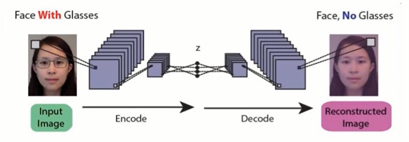
2) Image colourization – Autoencoders maps circles and squares from an image to the same image with red and blue, respectively. It is useful in converting any black and white picture to a coloured image.

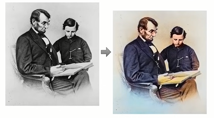
3) Feature variation – It extracts only the required features of an image and generates the output by removing any noise or unnecessary interruption.

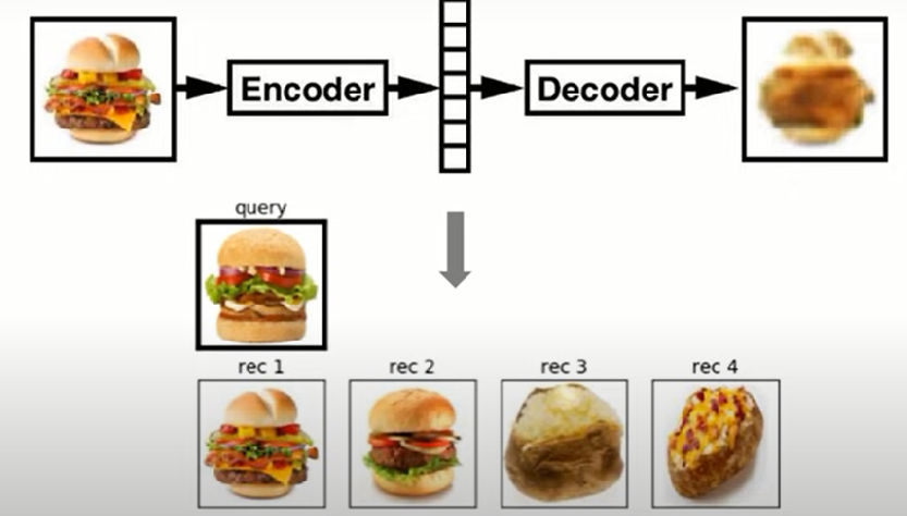
4) Image Search – Deep autoencoders can compress images into 30 number vector images. Image search becomes a matter of application where a search engine will compress an image and compare the vector to index and translate to a matching image.

Hands-On Implementation of Anomaly Detection model using Autoencoders

About Dataset

We will be using ECG dataset throughout this article. ECG stands for Electrocardiogram. It checks how your heart is functioning by measuring the electrical activities of your heart. Ian electrical pulse travels through the heart in each heartbeat, creating muscles to squeeze and pump blood to the heart. It carries the electrical impulse that helps the doctor know if the heart is pumping normally or strange. So we will take this dataset and build an anomaly detector using Autoencoder. Download the dataset zip folder and extract it from here.

Loading Libraries

We import the important libraries like pandas and numpy to play with data(data preprocessing and common mathematical operations), matplotlib for data visualization. We use Keras API built on top of TensorFlow for model building.

import pandas as pd
import numpy as np
import matplotlib.pyplot as plt
import matplotlib as mpl
import tensorflow as tf
from tensorflow.keras.models import Model
from sklearn.model_selection import train_test_split
from sklearn.preprocessing import MinMaxScaler, StandardScaler
mpl.rcParams['figure.figsize'] = (10, 5)
mpl.rcParams['axes.grid'] = False

We combine the train and test files to load the dataset and save the result in another file. For this, use the same cat command in jupyter notebook or google collab, and then we load the data. Data does not have a header, so we give it as a None otherwise, it uses the first row as a header. The data has 5000 rows and 140 columns, where the first column is our target column.

!cat "/ECG5000_TRAIN.txt" "/ECG5000_TEST.txt" > ecg_final.txt
df = pd.read_csv("ecg_final.txt", sep='  ', header=None)
df.shape

Basic Preprocessing

Pandas give the default name as numeric to the column name, so we cannot do any processing because pandas do not allow slice and dice if we have only numeric in the column name. So, we are adding any prefix to the column name to do slice and dice on columns.

df = df.add_prefix('c')
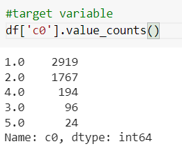
df['c0'].value_counts()

Suppose we see the number of records in each category using the value counts function. In that case, we see one has more number of observations so that we will take the first category into the normal data and combine the data from the second category to the fifth as abnormal.

Train-Test Splitting and Scaling the data

Before separating the data as normal and abnormal, we split the data into train and test sets. Neural networks give a good performance when data is scaled on a common scale, so we normalize the data.

x_train, x_test, y_train, y_test = train_test_split(df.values, df.values[:,0:1], test_size=0.2, random_state=111)

scaler = MinMaxScaler()
data_scaled = scaler.fit(x_train)
train_data_scaled = data_scaled.transform(x_train)
test_data_scaled = data_scaled.transform(x_test)

Separate Anomaly and Normal Data

Now we will split the training data into normal data and anomaly data. We know how to split these two datasets based on the value train data scale means the first category in normal data and the remaining category data in anomaly data. And the same applies to test data.

normal_train_data = pd.DataFrame(train_data_scaled).add_prefix('c').query('c0 == 0').values[:,1:]
anomaly_train_data = pd.DataFrame(train_data_scaled).add_prefix('c').query('c0 > 0').values[:, 1:]
normal_test_data = pd.DataFrame(test_data_scaled).add_prefix('c').query('c0 == 0').values[:,1:]
anomaly_test_data = pd.DataFrame(test_data_scaled).add_prefix('c').query('c0 > 0').values[:, 1:]

Now the training dataset has its own normal and anomaly dataframe. This is an 80-20 split. The dataset is not highly imbalanced that we need to do anything, but anyway, like for Autoencoder, we will train only with a normal dataset. An anomaly dataset will only be used for validation and finding inference.

Data Visualization

Data visualization is vital to understanding the relationship between two or more variables. So that we can see how the data differs, let us first plot the normal data.

plt.plot(normal_train_data[0])
plt.plot(normal_train_data[1])
plt.plot(normal_train_data[2])
plt.title("Normal Data")
plt.show()

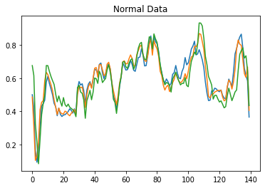
We plot the first three columns. At an initial level, it is dropped because ECG measurement starts from there, and then it moves in a normal way. Now let us plot take anomaly data on the contrary.

plt.plot(anomaly_train_data[0])
plt.plot(anomaly_train_data[1])
plt.plot(anomaly_train_data[2])
plt.title("Anomaly Data")
plt.show()

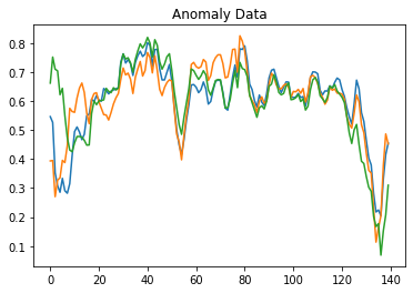
By observing the above graphs difference between normal and anomaly data can be easily understood. If you remember about the term reconstruction error we discussed above, we will use it to identify and differentiate anomaly and normal data.

Modelling

To create an autoencoder model, there are two ways. One is to use Sequential modelling provided by Keras API on top of TensorFlow. First, we add the encoding layer, decoding layers and one intermediate layer. It converts the data from a higher dimension into a lower dimension(). And then, to reconstruct the data back, it uses an upsampler. The below code snippet defines this architecture.

model = tf.keras.Sequential()
model.add(tf.keras.layers.Dense(64, activation="relu"))
model.add(tf.keras.layers.Dense(32, activation="relu"))
model.add(tf.keras.layers.Dense(16, activation="relu"))
model.add(tf.keras.layers.Dense(8, activation="relu"))
model.add(tf.keras.layers.Dense(16, activation="relu"))
model.add(tf.keras.layers.Dense(32, activation="relu"))
model.add(tf.keras.layers.Dense(64, activation="relu"))
model.add(tf.keras.layers.Dense(140, activation="sigmoid"))

The difference between input and output is reconstruction error which will be very high compared to normal data, which is used to differentiate between normal and anomaly data.

The other way that we will use is subclassing or Model subclassing. Why we use it is because it tells us to use encoder and decoder separately easily. suppose If we want this Model only for compressing the data, then I can only use encoder. Hence, it allows using a model in multiple different ways. Below is a code snippet and an explanation of it.

class AutoEncoder(Model):
  def __init__(self):
    super(AutoEncoder, self).__init__()
    self.encoder = tf.keras.Sequential([
                  tf.keras.layers.Dense(64, activation="relu"),
                  tf.keras.layers.Dense(32, activation="relu"),
                  tf.keras.layers.Dense(16, activation="relu"),
                  tf.keras.layers.Dense(8, activation="relu")
              ])
    self.decoder = tf.keras.Sequential([
                  tf.keras.layers.Dense(16, activation="relu"),
                  tf.keras.layers.Dense(32, activation="relu"),
                  tf.keras.layers.Dense(64, activation="relu"),
                  tf.keras.layers.Dense(140, activation="sigmoid")
              ])
  def call(self, x):
    encoded = self.encoder(x)
    decoded = self.decoder(encoded)
    return decoded

Explanation ~ Above, we create a class and create a constructor, and then we create an encoder in the same way of decreasing layer order and 8 units are bottleneck layers. Then we have a decoder that does upsampling of the data that is downsampled by an encoder and finally, the output is 140 units. depending on the problem statement number of units changes. The final activation function is sigmoid. The call function calls the encoder and passes the input data and the encoded data is passed to the decoder. So this Autoencoder is a class and when I run this class it will return the final model object which contains an encoder, bottleneck layer, and a decoder.

Compile and train the Model

We are adding the Early Stopping phenomenon which terminates the training if the validation loss is not decreasing after two epochs. Then we compile the Model using Adam optimizer. we use MAE(mean absolute error) as a loss function. Now we pass the train data to the Model (we pass it two times because it is a mandatory field so pass a dummy Y values). We add 50 epochs but due to early stopping, it will not run too many epochs. If you are using time-series data then the order is important so you have to set shuffle to False.

model = AutoEncoder()
early_stopping = tf.keras.callbacks.EarlyStopping(monitor="val_loss", patience=2, mode="min")
model.compile(optimizer='adam', loss="mae")
history = model.fit(normal_train_data, normal_train_data, epochs=50, batch_size=120,
                    validation_data=(train_data_scaled[:,1:], train_data_scaled[:, 1:]),
                    shuffle=True,
                    callbacks=[early_stopping]
                    )

Model Evaluation

In Autoencoders difference between training loss and validation loss is high. It does not mean that Model is underfitting. The reason is in the validation function I am giving both the normal data and abnormal data against training data as normal data so you will see this kind of behaviour which is completely fine that’s why we are having early stopping. I can get my encoder and decoder output separately.

encoder_out = model.encoder(normal_test_data).numpy() #8 unit representation of data
decoder_out = model.decoder(encoder_out).numpy()

First, we will plot the performance on Normal data which is first-class data.

plt.plot(normal_test_data[0], 'b')
plt.plot(decoder_out[0], 'r')
plt.title("Model performance on Normal data")
plt.show()

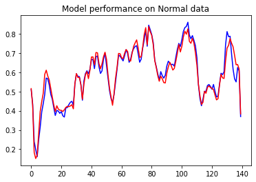
As discussed there will be a very little reconstruction error on Normal data which we can see in the above graph. The difference between both the red and blue lines is very less. what if I pass the anomaly test data.

encoder_out_a = model.encoder(anomaly_test_data).numpy() #8 unit representation of data
decoder_out_a = model.decoder(encoder_out_a).numpy()

plt.plot(anomaly_test_data[0], 'b')
plt.plot(decoder_out_a[0], 'r')
plt.title("Model performance on Anomaly Data")
plt.show()

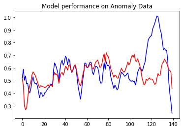
The top is anomaly test data and the red one is decoder output. if you see that the reconstruction error over here is pretty high. Now we got a very good model.

Calculate Loss

Now we will define our loss like threshold loss for our Model which gives us an output error between input and output. we define the Keras loss function over mean absolute error and plot it in form of a histogram.

reconstruction = model.predict(normal_test_data)
train_loss = tf.keras.losses.mae(reconstruction, normal_test_data)
plt.hist(train_loss, bins=50)

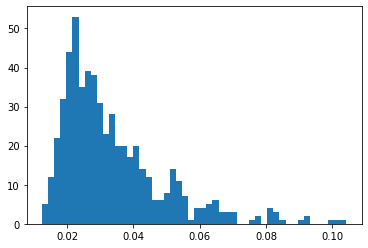
If you see the X-axis then most of the values lie below 0.5. there are a few anomalies because we cannot have a 100% perfect model. This is how the error looks like between normal data and reconstructed data. Now we want to set a threshold from which we can tell that value above it is anomalies and below it is normal data so we take the mean of training loss and multiply it with second standard deviation. The threshold should be set as per business standards.

threshold = np.mean(train_loss) + 2*np.std(train_loss)
reconstruction_a = model.predict(anomaly_test_data)
train_loss_a = tf.keras.losses.mae(reconstruction_a, anomaly_test_data)

plt.hist(train_loss_a, bins=50)
plt.title("loss on anomaly test data")
plt.show()

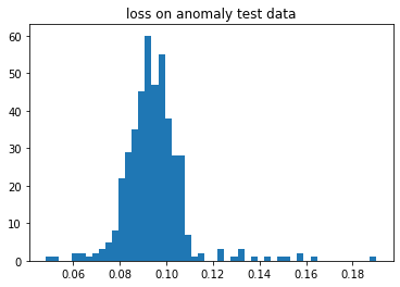
If you saw the above graph then most of the data were below 0.5 and if we plot histogram on anomaly test data loss then most of the data lies above 0.5. Observe the separation between normal data loss and anomaly data loss; hence, we got a very good model.

Plot Normal and anomaly Loss together

To get a better idea of how both losses together look like let us plot both the loss along with the threshold. So we pass the normal training loss and anomaly loss in a separate histogram on a single graph. we are drawing a vertical line on the graph which is the threshold for better visualization.

plt.hist(train_loss, bins=50, label='normal')
plt.hist(train_loss_a, bins=50, label='anomaly')
plt.axvline(threshold, color='r', linewidth=3, linestyle='dashed', label='{:0.3f}'.format(threshold))
plt.legend(loc='upper right')
plt.title("Normal and Anomaly Loss")
plt.show()

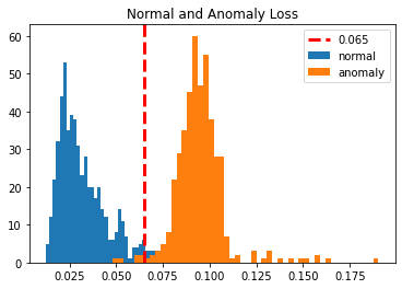
Now if you see a mean anomaly loss then earlier it was 33 percent but not it is 90 percent which is way far but the standard deviation will be close. Now we have a very good understanding of model performance so let us see how many false positives and false negatives are there so that we can define the average model performance.

How well does it predict Normal Class?

Anomaly data is data above to threshold so we use TensorFlow max function to find the values that are in anomaly data.

preds = tf.math.less(train_loss, threshold)
tf.math.count_nonzero(preds)

Among 563 total records, it predicts 536 values correctly so we can say that Model is 95 per cent accurate in predicting normal class.

How well does it perform on Anomaly data?

Now we use a greater function to find the count of values that are greater than a threshold which is anomalies.

preds_a = tf.math.greater(train_loss_a, threshold)
tf.math.count_nonzero(preds_a)

From 437 total records 431, it has predicted accurately means the final Model is 90 to 95 per cent accurate in predicting the new points.

End Notes

Hurray! we have made our first autoencoder model from scratch for anomaly detection which is working pretty decent on new unseen data. You can use different architecture like LSTM, convolutional 1-d, etc but this is a base model only to make you understand the working and requirement of Autoencoder in today’s data world and how does it manage to give better results than other models like PCA, isolation forest.

I hope that it was easy to catch up with each heading we have discussed in this guide. you can post your doubts in the comment section below 👇, and can connect with me.👍

Image Sources

• Towards Data Science(Applications of Autoencoders)
• Autoencoder Architecture at TDS
• Some Images are code screenshots and Graph Plots

Connect with me on Linkedin

Check out my other articles here and on Blogspot

Thanks for giving your time!

Raghav Agrawal

I am a software Engineer with a keen passion towards data science. I love to learn and explore different data-related techniques and technologies. Writing articles provide me with the skill of research and the ability to make others understand what I learned. I aspire to grow as a prominent data architect through my profession and technical content writing as a passion.