CONVOLUTIONAL NEURAL NETWORK(CNN)

This article was published as a part of the Data Science Blogathon.

To understand Convolutional Neural networks, we first need to know What is Deep Learning?

Deep Learning is an emerging field of Machine learning; that is, it is a subset of Machine Learning where learning happens from past examples or experiences with the help of ‘Artificial Neural Networks’.

Deep Learning uses deep neural networks, where the word ‘deep’ signifies the presence of more than 1 or 2 hidden layers apart from the input and output layer.

What is an Artificial Neural Network?

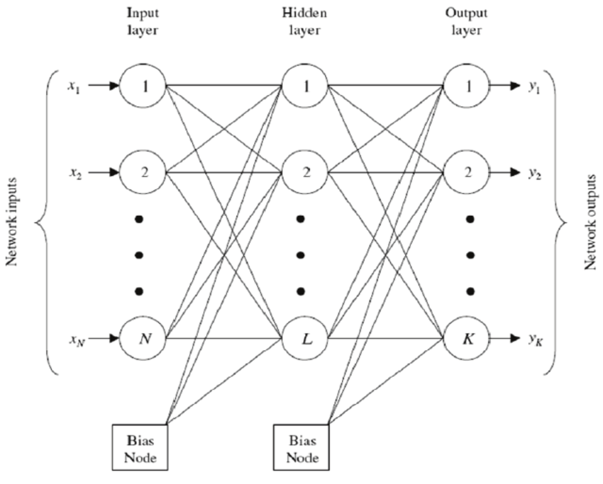
Artificial neural networks are made up of neurons, which are the core processing units of the network. For better understanding, refer to the diagram below:

In the given diagram, first, we have the ‘INPUT LAYER’, where the neurons are fed with training observations. Then in between is the ‘HIDDEN LAYER‘ that performs most of the computations required by our network. Lastly, the ‘OUTPUT LAYER‘ predicts the final output extracted from the previous two layers.

source: researchgate.net

How does this neural network work?

• For instance, if an image is passed as input, with N X N pixels, each pixel is fed as input to each neuron of the first layer.
• Neurons of one layer are connected to the following layers through ‘channels’.
• Each of these channels is assigned a numerical value called ‘weight’.
• The inputs (x₁, x₂, …… x_n) are multiplied by their corresponding weights, and their sum is sent to the neurons in the hidden layer.
• Each of these neurons is associated with a numerical value called the ‘Bias’, further added to the input sum.
• This value is then passed through a threshold function called the ‘Activation function’, which determines whether the particular neuron will get activated or not.
• The activated neuron transmits data to neurons of the next layer over channels.
• Thus, data is propagated through the network, and the neuron with the highest value determines the output.
• Output= f(sigma w _i*x_i)+Bias ,where f is the activation function.

Types of Deep Neural Network:

• Artificial Neural Network
• Multi-Layered Perceptron
• Recurrent Neural Network
• Convolutional Neural Network

CONVOLUTIONAL NEURAL NETWORK(CNN):

It is a class of deep neural networks that extracts features from images, given as input, to perform specific tasks such as image classification, face recognition and semantic image system. A CNN has one or more convolution layers for simple feature extraction, which execute convolution operation (i.e. multiplication of a set of weights with input) while retaining the critical features (spatial and temporal information) without human supervision.

Why do we need CNN over ANN?

CNN is needed as it is an important and more accurate way for image classification problems. With Artificial Neural Networks, a 2D image would first be converted into a 1-dimensional vector before training the model.

Also, with an increase in the size of the image, the number of training parameters would increase exponentially, resulting in loss of storage. Moreover, ANN cannot capture the sequential information required for sequence data.

Thus, CNN would always be a preferred way for dealing with 2D image classification problems because of its ability to deal with images as data, thereby providing higher accuracy.

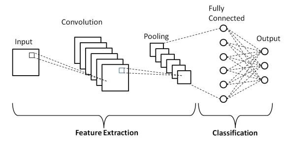
The architecture of CNN:

 

source: medium

The three primary layers that define the structure of a convolutional neural network are:

1)Convolution layer:

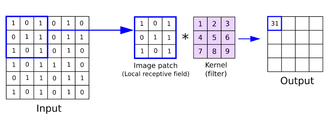
This is the first layer of the convolutional network that performs feature extraction by sliding the filter over the input image. The output or the convolved feature is the element-wise product of filters in the image and their sum for every sliding action.

The output layer, also known as the feature map, corresponds to original images like curves, sharp edges, textures, etc.

In the case of networks with more convolutional layers, the initial layers are meant for extracting the generic features while the complex parts are removed as the network gets deeper.

The image below shows the convolution operation.

source: analyticsindiamag.com

2)Pooling Layer:

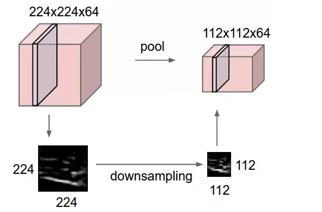
The primary purpose of this layer is to reduce the number of trainable parameters by decreasing the spatial size of the image, thereby reducing the computational cost.

The image depth remains unchanged since pooling is done independently on each depth dimension. Max Pooling is the most common pooling method, where the most significant element is taken as input from the feature map. Max Pooling is then performed to give the output image with dimensions reduced to a great extent while retaining the essential information.

source: computer science wiki

3)Fully Connected Layer:

The last few layers which determine the output are the fully connected layers. The output from the pooling layer is Flattened into a one-dimensional vector and then given as input to the fully connected layer.

The output layer has the same number of neurons as the number of categories we had in our problem for classification, thus associating features to a particular label.

After this process is known as forwarding propagation, the output so generated is compared to the actual production for error generation.

The error is then backpropagated to update the filters(weights) and bias values. Thus, one training is completed after this forwarding and backward propagation cycle.

IMPLEMENTATION

Now, let’s implement CNN by taking an example of classifying an image as a dog or cat. Dataset can be downloaded from https://www.kaggle.com/c/dogs-vs-cats/data

import cv2

import os

import numpy as np

import pandas as pd

import sklearn

import keras

from keras.models import Sequential

import tensorflow as tf

from keras.preprocessing.image import ImageDataGenerator

#Data Preprocessing

train_datagen = ImageDataGenerator(rescale = 1./255,

                                   shear_range = 0.2,

                                   zoom_range = 0.2,

                                   horizontal_flip = True)

train_generator = train_datagen.flow_from_directory(r"C:dogs vs catstrain",

                                                 target_size = (64,64),

                                                 batch_size = 32,

                                                 class_mode = 'binary')

test_datagen=ImageDataGenerator(rescale=1./255)

validation_generator = test_datagen.flow_from_directory(r"C:dogs vs catstest",

                                            target_size = (64,64),

                                            batch_size = 32,

                                            class_mode = 'binary')

## Build the CNN Model

#initialize the model

cnn=tf.keras.models.Sequential()

#Convolution

cnn.add(tf.keras.layers.Conv2D(filters=32,kernel_size=3,activation='relu', input_shape=[64,64,3]))

#Pooling

cnn.add(tf.keras.layers.MaxPool2D(pool_size=2,strides=2))

#Adding one more Convolution layer

cnn.add(tf.keras.layers.Conv2D(filters=32,kernel_size=3,activation='relu'))

# Adding one more Pooling Layer

cnn.add(tf.keras.layers.MaxPool2D(pool_size=2,strides=2))

#Flatening

cnn.add(tf.keras.layers.Flatten())

#Full Connection Layer

cnn.add(tf.keras.layers.Dense(units=128,activation='relu'))

#Full Connection Layer

cnn.add(tf.keras.layers.Dense(units=128,activation='relu'))

#compile the model

cnn.compile(optimizer='adam',loss='binary_crossentropy',metrics=['accuracy'])

cnn.summary()

The above output shows that the number of trainable parameters is 813,217, which can be reduced by adding more convolutional and pooling layers. With the increase in the number of layers, the features extracted will be more specific.

cnn.fit(x= train_generator , validation_data=validation_generator,epochs=25)

Thus, we get accuracy up to 90%, which can further be increased by adding more layers before the fully connected layer.

We have performed 25 epochs; you can further increase the number of epochs to train your model.

Read more articles on our blog.

The media shown in this article is not owned by Analytics Vidhya and are used at the Author’s discretion.