This article was published as a part of the Data Science Blogathon.
Introduction
As a part of writing a blog on the ML or DS topic, I selected a problem statement from Kaggle which is Microsoft malware detection. Here this blog explains how to solve the problem from scratch.
In this blog I will explain to you, how I deal with is the problem and use Microsoft malware detection.
Here I am applying the applied ML algorithm and statistics to solve the problem.
Content
- What is malware?
- Business problem
- Data overview
- Mapping into an ML problem
- EDA(exploratory data analysis)
- Extract feature
- Encoding feature
- Multivariate Analysis
- Apply ML model
- Final model
- Compare model
- Conclusion
- Reference
What is Malware?
Malware is intrusive-software that is designed to damage and destroy computers and computer systems and Malware is a contraction for “malicious software.” Examples of common malware include viruses, worms, Trojan viruses, spyware, adware, and ransomware.
Source:- click here.

Business Problem
In the past few years, the malware industry has grown very rapidly that, the syndicates invest heavily in technologies to evade traditional protection, forcing the anti-malware groups/communities to build more robust software to detect and terminate these attacks. The major part of protecting a computer system from a malware attack is to identify whether a given piece of file/software is malware.
This dataset contains 9 classes of malware.
Source: https://www.kaggle.com/c/malware-classification
Data overview
In this section, we understood the data that we have. So for each malware. We have given the two types of files. The first file is the.ASM file. And the second one is the .bytes files.
For more about.ASM files, https://www.reviversoft.com/file-extensions/asm
So ASM means assembly language code file, let’s assume you have to write code in C++ and C++ compiler take this raw code and convert it into an ASM file, and then something called is an assembler and it converts into bytes files and this file contains only 0’s and 1’s
.asm files contain this type of keyword like ‘pop’, ‘jump’, ‘push’, ‘move’, etc.
And bytes file(the raw data contains the hexadecimal representation of the file’s binary content, without the PE header) contain hexadecimal values and where the value lies between 00 to FF
Here we have a total of 200GB data where 50 GB data of bytes files and 150 GB is .asm file.
So the name of the nine malware is as follow:
- Ramnit
- Lollipop
- Kelihos_ver3
- Vundo
- Simda
- Tracur
- Kelihos_ver1
- Obfuscator.ACY
- Gatak
.ASM File
.text:00401030 56							       push    esi
.text:00401031 8B F1							       mov     esi, ecx
.text:00401043 74 09							       jz      short loc_40104E
.text:00401045 56							       push    esi
.text:00401046 E8 6C 1E	00 00						       call    ??3@YAXPAX@Z    ; operator delete(void *)
.text:0040104B 83 C4 04							       add     esp, 4
.text:0040104E
.text:0040104E						       loc_40104E:			       ; CODE XREF: .text:00401043j
.text:0040104E 8B C6							       mov     eax, esi
.text:00401050 5E							       pop     esi
.text:00401051 C2 04 00							       retn    4
.bytes file
6A 04 68 00 10 00 00 68 66 3E 18 00 6A 00 FF 15

D0 63 52 00 8B 4C 24 04 6A 00 6A 40 68 66 3E 18

00 50 89 01 FF 15 9C 63 52 00 50 FF 15 CC 63 52

00 B8 07 00 00 00 C2 04 00 CC CC CC CC CC CC CC

B8 FE FF FF FF C3 CC CC CC CC CC CC CC CC CC CC

B8 09 00 00 00 C3 CC CC CC CC CC CC CC CC CC CC

B8 01 00 00 00 C3 CC CC CC CC CC CC CC CC CC CC

B8 FD FF FF FF C2 04 00 CC CC CC CC CC CC CC CC

8B 4C 24 04 8D 81 D6 8D 82 F7 81 F1 60 4F 15 0B

23 C1 C3 CC CC CC CC CC CC CC CC CC CC CC CC CC

8B 4C 24 04 8B C1 35 45 CF 3F FE 23 C1 25 BA 3D

C5 05 C3 CC CC CC CC CC CC CC CC CC CC CC CC CC

8B 4C 24 04 B8 1F CD 98 AE F7 E1 C1 EA 1E 69 D2

FA C9 D6 5D 56 8B F1 2B F2 B8 25 95 2A 16 F7 E1

8B C1 2B C2 D1 E8 03 C2 C1 E8 1C 69 C0 84 33 73

1D 2B C8 8B C1 85 F6 74 06 33 D2 F7 F6 8B C2 5E

8B 4C 24 04 8B D1 8D 81 D6 8D 82 F7 81 F2 60 4F
Mapping into an ML problem
So given the files, We have to classify one of the nine classes, which lets us first convert it into the proper machine learning problem.
So it is the multiclass–classification problem.
For this problem performance metrics, we use is the multiclass log loss, and we also–use precision and recall metrics, which give a better idea about how our modes are, precise.
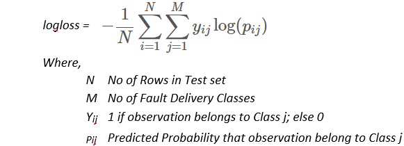
Multiclass log loss returns the probability of each class.
For more about the log, loss click here.
EDA
So in this section will perform a bunch of the EDA(exploratory data analysis) operations.
So let’s go and do EDA. So the first thing that we do here is separate bytes files from the ASM files. this problem is the imbalanced datasets so first, we are plotting histograms on the class labels.
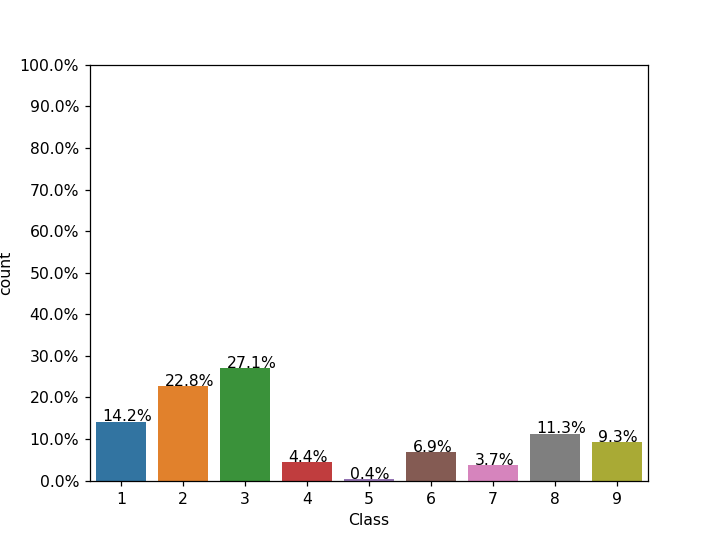
From this histogram of the class label, we can say that class 5 has very very few-data—points, and classes 2 and 3 have a good amount of data–points-available.
Extract Feature from .bytes files
So first look at a bytes file and do some feature engineering
Here we first look at the file size as a feature and plot a box plot to understand this feature is useful or not to determine the class labels, if all class labels box plots is overlapping with each other then we can say this file size as a feature is not useful.
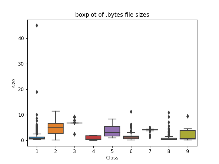
From the box plot, we can say that the file size feature is useful to determine the class label.
So our second things of feature extraction are as follows:
We know bytes files contain hexadecimal values and hexadecimal values lie between 00 to FF so we take all hexadecimal values as input values or features.
00,01,02,03,04,05,06,07,08,09,0a,0b,0c,0d,0e,0f,10,11,12,13,14,15,16,17,18,19,1a,1b,1c,1d,1e,1f,20,21,22,23,24,25,26,27,28,29,2a,2b,2c,2d,2e,2f,30,31,32,33,34,35,36,37,38,39,3a,3b,3c,3d,3e,3f,40,41,42,43,44,45,46,47,48,49,4a,4b,4c,4d,4e,4f,50,51,52,53,54,55,56,57,58,59,5a,5b,5c,5d,5e,5f,60,61,62,63,64,65,66,67,68,69,6a,6b,6c,6d,6e,6f,70,71,72,73,74,75,76,77,78,79,7a,7b,7c,7d,7e,7f,80,81,82,83,84,85,86,87,88,89,8a,8b,8c,8d,8e,8f,90,91,92,93,94,95,96,97,98,99,9a,9b,9c,9d,9e,9f,a0,a1,a2,a3,a4,a5,a6,a7,a8,a9,aa,ab,ac,ad,ae,af,b0,b1,b2,b3,b4,b5,b6,b7,b8,b9,ba,bb,bc,bd,be,bf,c0,c1,c2,c3,c4,c5,c6,c7,c8,c9,ca,cb,,cf,d0,d1,d2,d3,d4,d5,d6,d7,d8,d9,da,db,dc,dd,de,df,e0,e1,e2,e3,e4,e5,e6,e7,e8,e9,ea,eb,ec,ed,ee,ef,f0,f1,f2,f3,f4,f5,f6,f7,f8,f9,fa,fb,fc,fd,fe,ff
Apply a pixel feature on bytes files
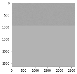
Here pixel basically means we take each file and we convert it into an image and then we use the first 100 pixels from the image as an input value.
Refer: more about it
Encoding Feature
Now we have features, For encoding a feature we apply a bi-gram BOW(bag-of-word), Let’s first understand BOW,
So BOW means we take each bytes file and we simply count how many times our features 00, 01, 02… occurs, and bi-gram means we take features and convert into in pair of features 00 01, 01 02, 02 03… and then we count how many time it occurs.
To know more about BOW.
Multivariate Analysis on .bytes file features
T-SNE is basically a dimension-reduction technique, so first, we take all data and convert it into a 2-dimension because using T-SNE we get the idea about it, our feature is useful to classify the class labels or not.
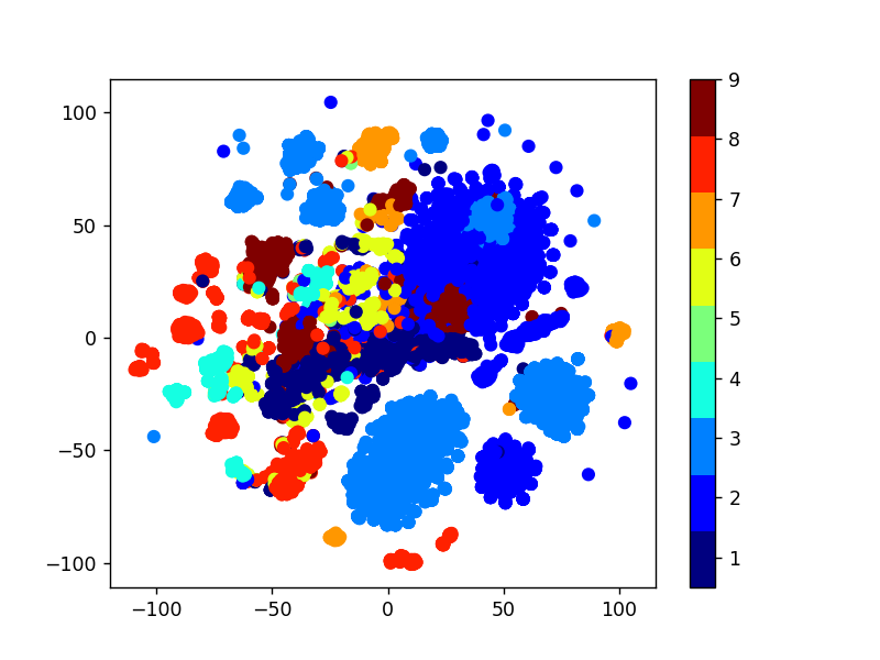
From the T-SNE we can say that our features are useful to classifying the class labels.
Apply ML model on .bytes files
1 Apply a Random model
We know our evaluation matric is a log-loss, and the log loss values lie between [0, infinity].
To find the highest value of log loss in our data we use a random model and we find a test and train log loss.
Random model as follows:-
First, we take our data and predict the class labels randomly, and–also we have an actual class label and we apply a multiclass log loss and we find the value of multiclass log loss on cv(cross-validation) data, and the value is 2.45.
This value is the very worst value for us so we have to try to minimize the log loss as much as we can do.
2 Apply KNN (K Nearest Neighbour Classification) on bytes files
Here we apply a KNN in our dataset which is a neighborhood-based–method, this is to take a K neighbor–point and predict the class labels.
Train and test loss is 0.078 and 0.245, here train and test loss differences are very high, hence we can say that our model is overfitting on the train data.
Observing the precision, we can say all data is well-classified for the all-class except class 5, it is because we have a very less amount of datapoint which belongs to class 5.
3. Apply a logistic regression on bytes files
We apply a logistic regression on the .bytes file.
Train and test loss are 0.1918 and 0.3168
Observing a log loss from the train, test data is little bit overfitting to the data.
But it is not classified all data–points. from the precision, we can say this is not predicting class 5 because of the less amount of data.
4 Apply Random Forest on bytes files
Here we apply an RF to the bytes data and it works well.
Train and test loss are 0.0342 and 0.0971
From the precision, we can say that it’s predicted almost every class label for class 5.
And from the recall, we can say that is the correct—classification for the almost class label. and looking from the log loss it’s well-fitted.
5 Apply XGBoost on bytes files
Now we apply an XGBoost on the data which is an ensemble model-based technique.
For more about it click here.
Train and test loss are 0.022 and 0.079, this loss is quite good than other models.
From the precision, we can say that it’s predicted almost every class label is–correct, even for class 5.
And From the recall, we can say that is the correct classification for the almost class label.
Extract Feature from .asm files
Now we extract the feature from the .asm file, All the files make up about 150 GB.
Here we extracted 52 features from all the .asm files which are important.
This file contains registers, keywords, opcodes, prefixes from these 4 parts of the file we extract a total of 52 features, and we include the file size–as a feature, so in total, we have 53 features here.
    prefixes = ['HEADER:','.text:','.Pav:','.idata:','.data:','.bss:','.rdata:','.edata:','.rsrc:','.tls:','.reloc:','.BSS:','.CODE']
    opcodes = ['jmp', 'mov', 'retf', 'push', 'pop', 'xor', 'retn', 'nop', 'sub', 'inc', 'dec', 'add','imul', 'xchg', 'or', 'shr', 'cmp', 'call', 'shl', 'ror', 'rol', 'jnb','jz','rtn','lea','movzx']
    keywords = ['.dll','std::',':dword']
    registers=['edx','esi','eax','ebx','ecx','edi','ebp','esp','eip']
Distribution of .asm file sizes
Now we plot a box plot a file size to understand this feature is useful or not to determine the class labels.

Source Author’s GitHub Profile
From the boxplot, we can say that file size as the feature is useful to classify our data.
Multivariate Analysis on .asm file features
For the multivariate analysis, we use the same concept which we use in bytes files, we apply a TSNE here to check whether these 53 features are useful to separate the data points or not.
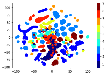
From the plot, there are many clusters for the different classes, hence we can say yes these features are useful to separate the labels
Apply the model on.ASM files
1 Apply a Random model on asm files:-
Here we know our performance matrix is a multiclass log loss, so we know log loss values lie between (0, infinity] here we know the low value but we don’t know a high value, using a random model we find a high value of log loss.
Hence the log loss on the test data for the random model is 2.493.
2 Apply KNN (K Nearest Neighbour Classification) on asm files
Here we apply a KNN in our dataset which is a neighborhood–base–technique, this is to take a K neighbor-point—and predict the class labels.
Train and test loss are 0.0476 and 0.089, here train and test loss differences are very high, hence we can say that our model is overfitting on the train data.
Observing the precision, we can say all data is well–classified for the all-class except class 5, it is because we have a very less amount of datapoint which belongs to class 5.
3. Apply a logistic regression on ams files
We apply a logistic regression on the .asm file.
Train and test loss are 0.781 and 0.742
The observing a log loss from the train, test data, is well-fitted.
But it is not classified all data points. from the precision, we can say this is not predicting class 5 because of the less amount of data.
And from the–recall, it’s not classified the–correct class label for the classes 5, 6, 7, and 9.
4 Apply Random Forest on bytes files
Here we apply an RF to the data and it works very well.
Train and test loss are 0.0271 and 0.0462
From the precision, we can say that it’s predicted almost every class label is correct, even for class 5.
And from the recall, we can say that is the correct classification for the almost class label.
And looking from the log loss it’s well-fitted
5 Apply XGBoost on bytes files
Here we apply an XGBOOST to the data and it works very well.
From the precision, we can say that it’s predicted almost every class label is correct, even for class 5.
Train and test loss are 0.0241 and 0.0371
And from the recall, we can say that is the correct classification for the almost class label.
And looking from the log loss it’s well-fitted, and this is also better than an RF model.
Final Model
Now we merge both files .asm and .bytes and Apply model which is performed better in–individual files and here the better model is XGboost.
Here we have a total of 66k features and this is a very challenging task for me, first, we apply a TSNE because it gives me an idea these features are how good to separate the labels
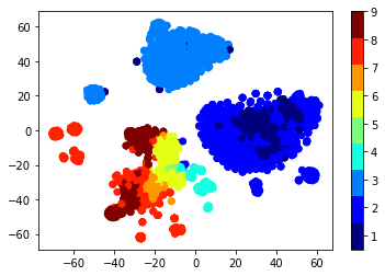
Now we can say these all feature is very useful to data—separation.
Here we did a multivariate on this .asm and bytes files feature and so we apply a T-SNE on this data with the different perplexity–values and we can observe–the nice cluster-of
Hence here we can this feature is helpful for separating—the data points.
Random Forest Classifier on final features
Here we apply an RF to the final data and it works
Train and test loss are 0.03143 and0.09624
From the precision, we can say that it’s predicted almost every class label for class 5.
And from the–recall, we can say that is the correct—classification for the almost class label.
And looking from the log loss it’s well-fitted. hence we can say RF work very–well for our data.
LGBMClassifier on final features
Here we know for both files our winner model is XGBOOST, but on the final feature, we apply lightgbm because our xgboost computing time is very high and lightgbm is a little bit fast than xgboost hence we apply LGBM here and both doing the same things.
Here we apply an LGBM to the final data and it works
From the precision, we can say that it’s predicted almost every class label for class 5.
And from can say that is the correct—classification for the almost class label.
And looking from the log loss it’s well-fitted, and this than an RF model. and we got a test loss is 0.01 here, hence LGBM/XGBOOST is working on our data.
Compare model
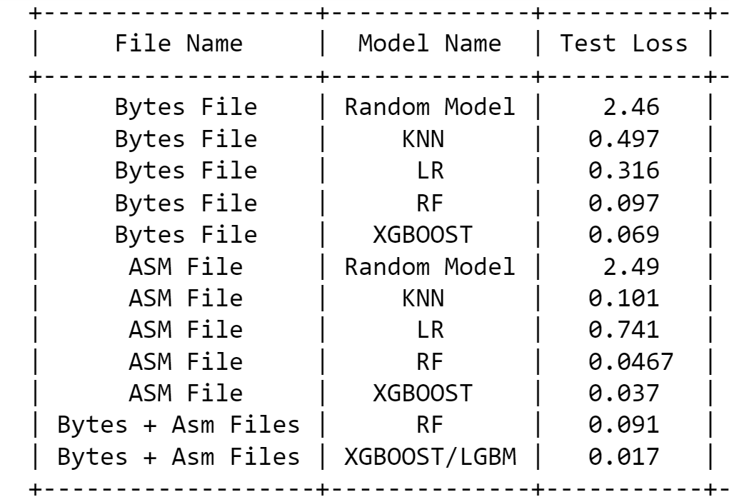
Conclusion
1. First, the given data is Microsoft malware data, and our task is to classify the given file has which type of malware to belong. here in data, we have 9 types of Microsoft malware detection available.
2. In our data 2 types of files are present, the first one is .bytes files and the second is .asm file.
A. In bytes files, they contain hexadecimal values
B. And in the .asm file, they contain some special keywords like pop, push, etc
3. Here we first unzip data and separate both types of files, and this data size is roughly 200GB. so it’s a very challenging thing here for us.
4. Here our approach is first we analyze the .bytes files and then we go to analyze the .asm files.
5. We first take a .bytes file and we know it contains a hexadecimal value and hexadecimal values lie between 00 to FF, so we apply simple bi-gram BOW and we do a simple count here for each file, and we also apply a pixel feature which means we first we convert each file into an image and we take a first 100 pixel.
6. We know the log-loss min value is 0 and max value is infinity, so first, we build one random model and find max log loss.
7. After the random model, we build a different model like LR, RF, KNN, xgboost, and we check which model gives a low log-loss.
8. Now we take the .asm file and we find some special 53 keywords which are very imp for the .asm file.
9. Here we also apply a different model like KNN, LR, RF, etc.
10. Now we combine both file features and apply an RF and XGBOOST/LGBM.
11. Using an XGBOOST/LGBM we got a test loss is 0.01.
Hope you enjoyed my article on Microsoft malware detection. If you have any doubts, comment below. Read more articles on the Analytics Vidhya blog.
Reference
https://towardsdatascience.com/malware-classification-using-machine-learning-7c648fb1da79
https://www.kaggle.com/c/microsoft-malware-prediction
https://www.appliedaicourse.com
Connect with me
The media shown in this article is not owned by Analytics Vidhya and are used at the Author’s discretion.


[…] post Microsoft Malware Detection appeared first on Analytics […]
[…] post Microsoft Malware Detection appeared first on Analytics […]