RFM and CLTV are two methods commonly utilized to analyze customer value. CLTV or CLV represents the amount of money a customer is expected to spend in your business during their lifetime and can be used to optimize your marketing efforts. RFM is commonly used for segmenting marketing strategies for different segments. CLTV helps you determine how much money you should spend acquiring new customers and retaining existing ones.
This article will walk you through how to use Pandas and Lifetimes modules to perform RFM and CLTV analyses in Python. The main focus will be CLTV, and we will create and add our RFM segments to our data so we can interpret our analysis of CLTV more effectively.
Let’s take a look at our data

Photo by Rick Mason on Unsplash
For today’s analysis, we will use the Online Retail 2 dataset. This data set contains all of the transactions recorded for an online retailer based and registered in the UK between 2009–12–01 and 2011–12–09. The retailer specializes in all-occasion gift items. Most of the retailer’s customers are wholesalers. The dataset has the following attributes:
InvoiceNo: Invoice number. Nominal. A 6-digit integral number is uniquely assigned to each transaction. If this code starts with the letter ‘C’, it indicates a cancellation.StockCode: Product (item) code. Nominal. A 5-digit integral number is uniquely assigned to each distinct product.Description: Product (item) name. Nominal.Quantity: The quantities of each product (item) per transaction. Numeric.InvoiceDate: Invoice date and time. Numeric. The day and time when a transaction was generated.UnitPrice: Unit price. Numeric. Product price per unit in sterling (£).CustomerID: Customer number. Nominal. A 5-digit integral number is uniquely assigned to each customer.Country: Country name. Nominal. The name of the country where a customer resides.
We will focus on purchases from UK customers between 2010–2011. Findings from Exploratory Data Analysis are as follows:
- · There are 485123 observation units, 8 attributes.
- · There are 130802 null values in Customer ID.
- · There are 3844 unique products.
- · There are 9288 returns.
- · There are a lot of outliers and negative values in Quantity and Price columns.
- · Most seen product in data set White Hanging Heart T-Light Holder.
- · The item that generated the most revenue is Paper Craft, Little Birdie.
Refer to the data pane via this link:
https://datapane.com/u/hokay/reports/VkGyql3/df-raw/?utm_medium=embed
Preparing the Data for Analysis

First, we drop null values on CustomerID. For outliers, since there are a lot of them, we don’t want to just drop all of them. Instead, we replace our outliers with ±1.5*IQR. Then we create our TotalPrice column which we will use to calculate our Monetary.
As stated in Lifetime’s module documentation, we have to put our data in a certain shape which consists of 4 columns and we will use CustomerIDas our index.
Frequency: Number of repeat purchases the customer has made.T: Customer’s first purchase and the end of the period under study. We will use weekly age on our analysis.Recency: The duration between a customer’s first purchase and their latest purchase.Monetary: Average value of a given customer’s purchases.
The last InvoiceDate available in the dataset is 2011–12–09. We have to select a proper analysis date since there have been 10 years since the last entry and then start preparing our columns. We will calculate customer lifetime(tenure) on a weekly scale that’s why we are dividing our recency and T columns by 7.
After cleaning and preparation this is how our data looks like:
https://datapane.com/u/hokay/reports/9ArDxM7/cltv-df/
Theory and Modelling
Before we dive into modelling, I want to talk about the theory behind our models. As stated before CLTV is the monetary value that a customer will bring to the company during the relationship and communication with a company. The most basic definition would be:
CTLV = Number of Transactions * Average Order Value
Since we are trying to predict our CLTV using probability with time projection we have to use 2 different models. The first one will be the Beta Geometric / Negative Binomial distribution model (BG/NBD) which will calculate the Expected Number of Transactions. And the second one will be Gamma Gamma Submodel which will calculate the Average Order Value.
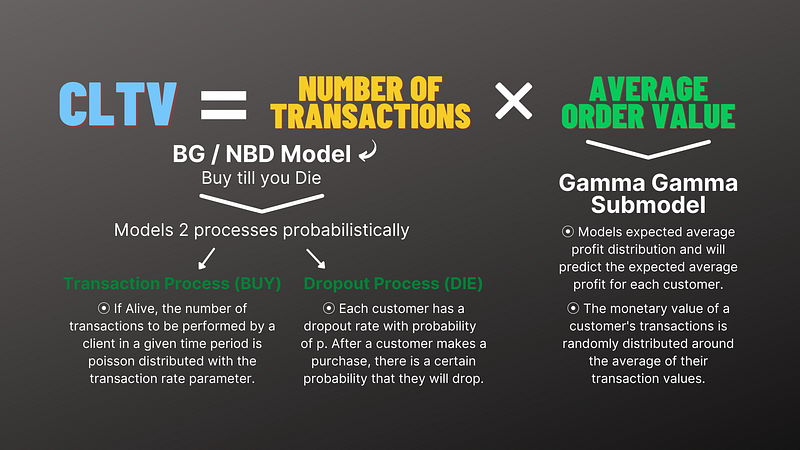
For modelling, we first fit our Frequency, Recency and T columns to BG/NBD model and Frequency, Monetary columns to our Gamma Gamma Submodel. Then we call the customer_lifetime_valuefunction on our Gamma model with BG/NBD as the first parameter. We also state our prediction length in months using time parameters. We state the frequency we used to calculate our Tenure which in this case is ‘W’ for weekly. After calculation, the values are still hard to interpret so we should put them on a scale. Using MinMaxScaler from the scikit-learn module we put our CLTV predictions on a 0 to 1 scale.
This is how our data looks like after calculating and scaling CLTV:
Refer to this link for the data pane: https://datapane.com/u/hokay/reports/BAmpowk/cltv-final/
RFM (Recency, Frequency, Monetary)

For better interpretation, we will add RFM segments to our CLTV table. This way we can compare our results from both methods. Let’s first create our RFM metrics, scores and segments.
This is how our RFM results look like:
https://datapane.com/u/hokay/reports/J35lD0A/rfm/
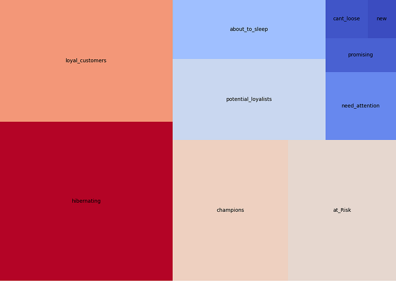
And this is the distribution of our RFM segments:
Bringing results together
Adding our RFM segments to our CLTV will give us a more solid foundation for our interpretation. We will also add 1 month and 12 months projections to our table which will lead us to see some interesting findings of the effect of monetary on CLTV modelling.
This is how our data looks like after adding RFM segments, 1-month CLTV and 12-months CLTV projections:
Refer to the data pane:
https://datapane.com/u/hokay/reports/E7PXrY7/final-triple/
CLTV Segmentation
Since we try to create better segmentation and marketing strategies based on RFM and CLTV we will also create segments based on our CLTV. ‘A’ for our best customers and ‘D’ for the worst.
Our final table looks like this:
https://datapane.com/u/hokay/reports/aAMZX63/final-segmented/
Discussion
I will discuss and interpret the results based on Pareto Principle. The Pareto principle states that for many outcomes, roughly 80% of consequences come from 20% of causes. In our case, we expect to see 80% of our income generated from our top 20% of customers. If we take a look at our segments from both analyses:
Refer to the below link for the data pane:
https://datapane.com/u/hokay/reports/O7vZKl7/top20rfmclv/
Most of our Champions, Loyal Customers and Potential Loyalists belong to A segment from our CLTV segmentation which makes sense. And if we look at how much value they brought to the business we can see Champions, Loyal Customers are generating roughly %80 of our income. For our top customers in these segments I would recommend the following:
- Organize loyalty programs.
- Advertise Limited Edition products.
- Provide special discounts.
- Tune recommendation systems.
- Pay attention to feedbacks of these groups.
- Provide special discounts and free shipments etc.
Caveats
Some important notes should be taken when using CLTV.
- The calculation represents a single period of time in which you performed the analysis.
- The churn rate comes from the whole audience, not personal.
- The profit comes from the whole audience, not personal.
- The total price is the dominant factor and crushes the frequency effect. It means if 2 customers brought the same amount, the frequency of their purchases doesn’t matter. This effect loses its dominance for predictions made for longer time periods. This effect can be seen on customers 16000 and 15601. If we look at 1-month predictions customer 16000 has higher CLTV than 15601 because of its monetary. But high frequency starts to show its effect on the longer-term and results in a higher CLTV for customer 15601 in the long run.
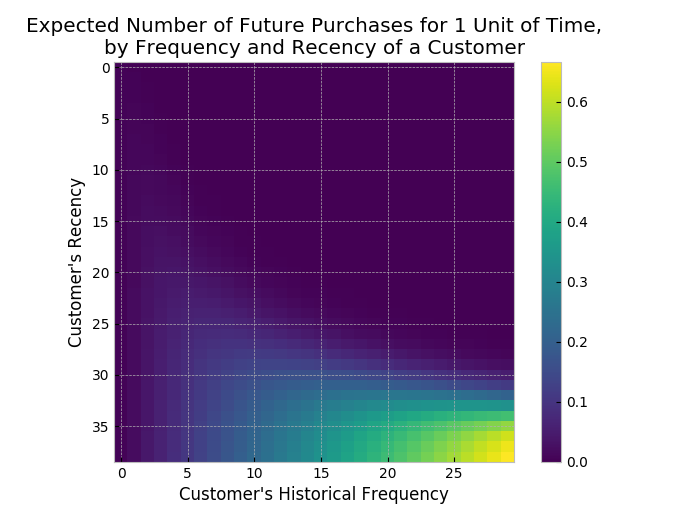
And since this is a model, there should be some metrics to evaluate the performance. To create a Frequency/Recency matrix that computes the expected number of transactions an artificial customer is to make in the next time period, given her recency and frequency:
from lifetimes.plotting import plot_frequency_recency_matrix
plot_frequency_recency_matrix(bgf)
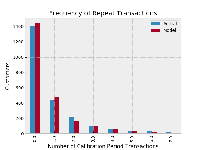
And to compare your data versus artificial data simulated with your fitted model’s parameters:
from lifetimes.plotting import plot_period_transactions
plot_period_transactions(bgf)
Conclusion
CLTV helps you determine how much money you can afford to spend acquiring new customers and retaining existing ones and RFM can be used to segment your customers to better target your marketing efforts. All the efforts to perform these analyses have only one goal which is to make better business decisions based on data. Using CLTV and RFM simultaneously and interpreting data based on both analyses can help businesses grow.
Performing these analyses using Python and Lifetimes modules is not the most important and complicated part. Knowing your business, having domain knowledge and using that knowledge to produce useful results from these analyses is the key to a business’s success.
References
- Measuring users is hard. Lifetimes makes it easy.
I’ve quoted “alive” and “die” as these are the most abstract terms: feel free to use your own definition of “alive” and…lifetimes.readthedocs.io - Veri Bilimi Okulu
Veri Bilimi Okulu | 18,400 followers on LinkedIn. Veri odaklı içerik üreticilerini bir araya getiren platform. | Veri…www.linkedin.com - Miuul
Miuul | 3,409 followers on LinkedIn. Miuul Original® Career Paths | Miuul yapay zeka çözümleri ve veri bilimi…www.linkedin.com - Projects/CRM Analytics/CLTV at master · h-okay/Projects
Various projects. Contribute to h-okay/Projects development by creating an account on GitHub.github.com
The media shown in this article is not owned by Analytics Vidhya and are used at the Author’s discretion.


