This article was published as a part of the Data Science Blogathon.
Introduction
In this article, we will learn to train Bidirectional Encoder Representations from Transformers (BERT) in order to analyze the semantic equivalence of any two sentences, i.e. whether the two sentences convey the same meaning or not. The following aspects are covered in the article:
- Why BERT?
- Data description
- Tokenization
- Encoding sentences, creating input mask and input type
- Model development
- Conclusion
Also, you would follow this article at a faster pace if you have at least a basic awareness of BERT. I have provided some quick readings about BERT at the bottom of this article for quickly refreshing BERT’s concepts. The rest of the aspects about BERT’s functioning, components and architectural aspects are covered by providing explanations, codes and architectural plots.
Why BERT?
BERT is a transformer-based language model pre-trained on a large amount of un-labelled text by jointly conditioning the left and the right context. There are multiple reasons for preferring BERT over models like/based on LSTM, GRU, Encoder-Decoder (Seq2seq) model, but I am listing only a few of them here.
- BERT is pre-trained on a very large amount of data
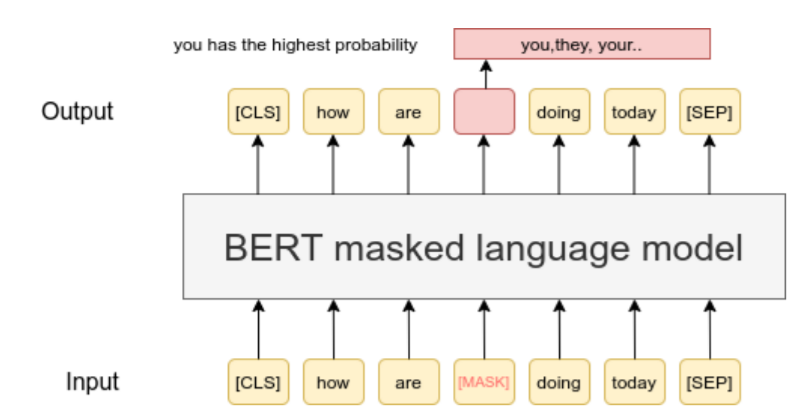
- It is truly bidirectional because of ‘Masked Language Modelling’, a novel approach that it leverages to train the language model.
Below is shown the figure describing Masked Language Modelling that BERT uses. It masks a few input words and computes the word probability for a pool of candidate words and assigns it the word with the highest probability.

source: https://www.sbert.net/examples/unsupervised_learning/MLM/README.html
- Efficient Tokenization: BERT tokenizes the text using WordPiece into sub-words which is more efficient than character-based or word-based tokenization leveraged in Elmo or ULMFit.
- BERT allows parallelization in training with is not possible in LSTM based models
So, let us start to analyze if semantic equivalence between sentences!
Data Description
I will be using the Microsoft Research Paraphrase Corpus (Dolan & Brockett, 2005) for building this model. The data can be found here: https://www.microsoft.com/en-us/download/details.aspx?id=52398
This is what the data looks like.
Tokenization
For the BERT model to understand this data, we will need to convert it into a suitable format. The first step to do that is to start by tokenization of the text. Since we are using a pre-trained model, we need to make sure that we use the same tokenization approach, vocabulary and index-mapping as was used while training the BERT model.
The code for creating the tokenizer that was used in the BERT model is written below:
bert_tokenizer = bert.tokenization.FullTokenizer(vocab_file=os.path.join(gs_folder_bert, "vocab.txt"), do_lower_case=True)
To confirm that this tokenizer is consistent with that used in the BERT model, we can check the size of the vocabulary.
From our knowledge about BERT, we know that the vocabulary size for BERT is 30522, and we have a match with that number. So, we can now move to our next broad step: data transformation
Encoding Sentences, Creating Input Mask and Input Type
When we send the sentences to our model to be compared for semantic equivalence, it needs to be sent in a very specific way. The model expects the two sentences to be concatenated by fulfilling the following two conditions.
Condition1: Each sentence needs to start with a [‘CLS’] token, i.e. conveying that it is a classification problem
Condition2: Each token should end with a [‘SEP’] token, i.e. a separator token
Below is a function that will add [‘SEP’] token to each of the sentences.
def SEP_encoding(s,bert_tokenizer):

tokens = list(bert_tokenizer.tokenize(s.numpy()))

tokens.append('[SEP]')

sep_encoded_sent=bert_tokenizer.convert_tokens_to_ids(tokens)

return sep_encoded_sent
Now we can create ragged tensor for both, sentence1 and sentence2 and the code used to do that is mentioned below:
sentence_1 = tf.ragged.constant([SEP_encoding(sent1,bert_tokenizer) for sent1 in data_train["sentence1"]])

sentence_2 = tf.ragged.constant([SEP_encoding(sent2,bert_tokenizer) for sent2 in data_train["sentence2"]])
Now that we have complied with one of the above conditions, let us now fulfil the second condition, i.e. we will add [‘CLS’] token to the ragged tensors that we created above.
After doing this, we will concatenate the ragged tensors to form a single input word id for each of the observations.
bert_cls = [bert_tokenizer.convert_tokens_to_ids(['[CLS]'])]*sentence_1.shape[0]

bert_input_word_ids = tf.concat([bert_cls, sentence_1, sentence_2], axis=-1)
source: https://arxiv.org/pdf/1810.04805.pdf (research paper)
The above figure shows the placement of the CLS token in the BERT input requirement schema. The hidden state corresponding to [CLS] will be used as sentence representation.
Now we move to the 2nd part of data transformation: Input mask.
We need to input the data in the model in a very specific manner. The model should be able to clearly distinguish between content and padding. Input mask allows us to do this. The input mask will have the same shape as the bert_input_word_ids. It will contain 1 at all the places where bert_input_word_ids is not padding. The code to do so is written below:
bert_input_mask = tf.ones_like(bert_input_word_ids).to_tensor()
The last aspect of transforming the data to make it suitable for modelling purpose is ‘input type’. It also has the same shape as bert_input_word_ids. Its purpose is that , inside the non-padded region, it will contain 0 or 1 depending upon the sentence that it is a part of.
bert_input_type_ids = tf.concat([bert_cls_type, type_sent1, type_sent2], axis=-1).to_tensor()
Now, I will write the above 3 aspects of data transformation in a single function to ease the functioning of the code and apply it to the dataset
def bert_sent_encoding(data, tokenizer):

# we create the raggedtensors and add ['SEP'] token to each sentence

sentence_1 = tf.ragged.constant([SEP_encoding(sent1, bert_tokenizer) for sent1 in data["sentence1"]])

sentence_2 = tf.ragged.constant([SEP_encoding(sent2, bert_tokenizer) for sent2 in data["sentence2"]])

# complying with the condition to add ['CLS'] token

bert_cls = [tokenizer.convert_tokens_to_ids(['[CLS]'])]*sentence_1.shape[0]

# creating input word ids, input mask and input type ids

bert_input_word_ids = tf.concat([bert_cls, sentence_1, sentence_2], axis=-1)

bert_input_mask = tf.ones_like(bert_input_word_ids).to_tensor()

bert_cls_type = tf.zeros_like(bert_cls)

type_sent1 = tf.zeros_like(sentence_1)

type_sent2 = tf.ones_like(sentence_2)
input_type_ids = tf.concat([bert_cls_type, type_sent1, type_sent2], axis=-1).to_tensor()
bert_input = {

'input_word_ids': bert_input_word_ids.to_tensor(),

'input_mask': bert_input_mask,

'input_type_ids': bert_input_type_ids}

return bert_input
We can apply the above function to our data (train, validation and test set) to create the final datasets that can be fed into our BERT model.
train = bert_sent_encoder(data['train'], tokenizer)

validation = bert_sent_encoder(data['validation'], tokenizer)

test = bert_sent_encoder(data['test'], tokenizer)


train_labels = data['train']['label']

test_labels = data['test']['label']

validation_labels = data['validation']['label']
After the data has been converted in the desired format, I will now proceed to the final step that we all had been waiting for: ‘Model development’.
Training BERT
A BERT model can be finalized by making a choice across the following 4 basic architectural aspects of BERT:
- Cased vs uncased
- Number of layers in the Encoder, indicated by the letter L in the model name
- Dimension of the output or embedding dimension, indicated by the letter H in the model name
- Number of multi-headed attention, indicated by the letter A in the model name
gs_folder_bert = "gs://cloud-tpu-checkpoints/bert/v3/uncased_L-12_H-768_A-12"
tf.io.gfile.listdir(gs_folder_bert)
hub_url_bert = "https://tfhub.dev/tensorflow/bert_en_uncased_L-12_H-768_A-12/3"
Let us start by downloading the pre-trained BERT configuration.
bert_config_file = os.path.join(gs_folder_bert, "bert_config.json")
config_dict = json.loads(tf.io.gfile.GFile(bert_config_file).read())
bert_configuration = bert.configs.BertConfig.from_dict(config_dict)
Based on the configuration finalized above, we get our BERT encoder and classifier using the following code:
BERT_classifier, BERT_encoder = bert.bert_models.classifier_model(bert_config, num_labels=2)
Now, we can even plot the BERT classifier’s architecture as shown below:
tf.keras.utils.plot_model(BERT_classifier, show_shapes=True, dpi=48)
The output of the above code is shown below:
Also, we can plot the BERT encoder by using the following piece of code:
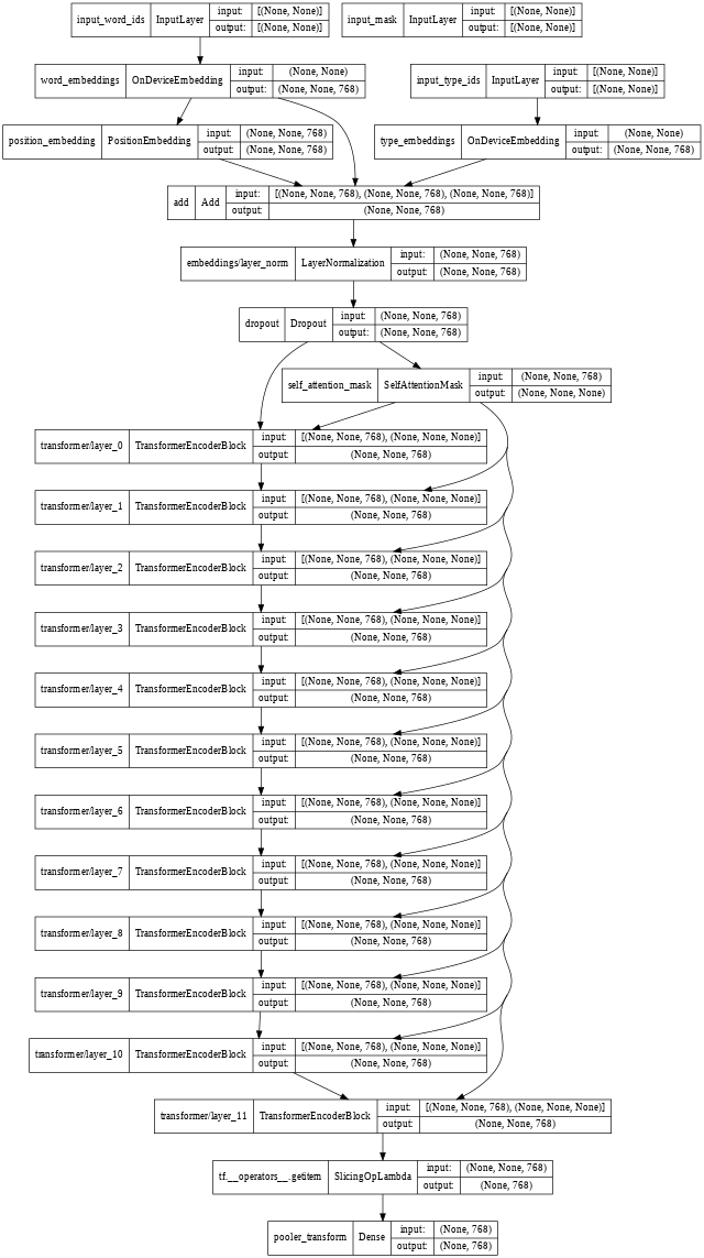
tf.keras.utils.plot_model(BERT_encoder, show_shapes=True, dpi=48)
The BERT encoder architecture can be seen below. We do see the input word ids, input mask and input type ids in the plot. Also, the word embeddings, position embeddings and type embedding are visible. It also shows the 12 encoder layers and the embedding dimension of 768 can also be noticed.
I advise that you pause for a while and minutely observe each of the layers displayed in the plot below. This will significantly boost your understanding of BERT’s architecture.

Now we will create our optimizer. BERT leverages Adam optimizer with weight decay. Also, I have created a learning rate schedule that will increase from 0 and then will finally decay to 0.
epochs = 5
batch_size = 32
size_eval_batch = 32
size_train_data = len(train_labels)
steps_per_epoch = int(size_train_data / batch_size)
num_train_steps = steps_per_epoch * epochs
warmup_steps = int(epochs * size_train_data * 0.1 / batch_size)
optimizer = nlp.optimization.create_optimizer(2e-5, num_train_steps=num_train_steps, num_warmup_steps=warmup_steps)
The parameters mentioned above should be optimized in order to get a model with good performance.
I will use accuracy as the metric of our performance and categorical cross-entropy as our loss function.
We are now at the last step. We will now train the model. The code to do so is shown below:
metrics = [tf.keras.metrics.SparseCategoricalAccuracy('accuracy', dtype=tf.float32)]
loss = tf.keras.losses.SparseCategoricalCrossentropy(from_logits=True)
BERT_classifier.compile(optimizer=optimizer,loss=loss,metrics=metrics)
BERT_classifier.fit(train, train_labels,validation_data=(validation, validation_labels), batch_size=batch_size , epochs=epochs)
Conclusion
The accuracy of the above model is 90%. which can be said to be a good performance. Here we have not performed hyper-parameter optimization, if we do so, this performance will further improve. Apart from measuring accuracy, we can also use other metrics such as F1-score, precision, recall and make inferences about the areas where the model is performing well and the kind of sentences on which we can improve further. I leave this as an assignment to you.
So, in this article, we saw how to prepare the data for the model. Then we looked at how to interpret BERT’s architecture and choose a model and import it. Then we trained that model on our data and looked at its accuracy. Now we look at two of its predictions.
We also look at some predictions that the model is making
example = bert_sent_encoding(
    data = {'sentence1':['Most of the Indians love cricket.'],
            'sentence2':['Cricket is loved by most of the Indians']},
    tokenizer=bert_tokenizer)
result = BERT_classifier(example, training=False)
result
The output of the sentence classifies the two sentences as the same with a probability of sentences being the same as 91.768%, which is a pretty high probability. Thus we can see that the model we created above works pretty well. Now I leave you to experiment with the BERT model that we created above!
Read more articles on BERT here.
Suggested Readings
Although I have studied BERT in my computer science course at IIT Kharagpur, I believe the following 2 sources are pretty useful:
- Jay Alamar’s blog: https://jalammar.github.io/illustrated-bert/
- Research paper: https://arxiv.org/abs/1810.04805
More advance and powerful transformer models can be referred from the hugging face documentation: https://huggingface.co/docs/transformers/index
About the Author
Parth Tyagi has done PGDBA (IIM Calcutta, IIT Kharagpur, ISI-Kolkata) and B.TECH from IIT DELHI and has ~4 years of work experience in Advanced Analytics. If you want to discuss any aspect of this article, feel free to reach out to me at:
- Linkedin: https://www.linkedin.com/in/parth-tyagi-4b867452/
- email-id: [email protected] | [email protected]
The media shown in this article is not owned by Analytics Vidhya and are used at the Author’s discretion.


