Blood Cell Detection in Image Using Naive Approach

This article was published as a part of the Data Science Blogathon.

The basics of object detection problems are how the data would look like. Now, this article will discuss the different deep learning architectures that we can use to solve object detection problems. Let us first discuss the problem statement that we’ll be working on.

Table of Contents

1. Understanding the Problem Statement Blood Cell Detection
2. Dataset Link
3. Naive Approach for Solving Object Detection Problem
4. Steps to Implement Naive Approach
   1. • Load the Dataset
      • Data Exploration
      • Prepare Dataset for Naive Approach
      • Create Train and Validation Set
      • Define Classification Model Architecture
      • Train the Model
      • Make Predictions
5. Conclusion

Understanding the Problem Statement Blood Cell Detection

Problem Statement

For a given set of images of blood cells, we have to detect the WBCs or the White Blood Cells in the images.
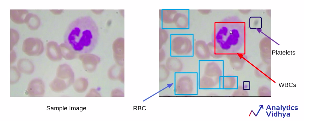
Now, here is a sample image from the data set. You can see that there are some red-shaded regions and a blue or a purple region, as you can see.

 Source: https://courses.analyticsvidhya.com/courses/take/Applied-Computer-Vision-using-Deep-Learning/lessons/13915281-understanding-the-problem-statement-blood-cell-detection

So in the above image, there are the red-shaded regions which are the RBCs or Red Blood Cells, and the purple-shaded regions, which are the WBCs,  and some small black highlighted portions, which are the platelets.

As you can see in this particular image, we have multiple objects and multiple classes.

We are converting this to a single class single object problem for simplicity. That means we are going to consider only WBCs.

Hence, just a single class, WBC, and ignore the rest of the classes. Also, we will only keep the images that have a single WBC.

So the images which have multiple WBCs will be removed from this data set. Here is how we will select the images from this data set.

So, we have removed image 2 and image 5 because image 5 has no WBC, whereas image 2 has 2 WBCs and the other images are a part of the data set. Similarly, the test set will also have only one WBC.

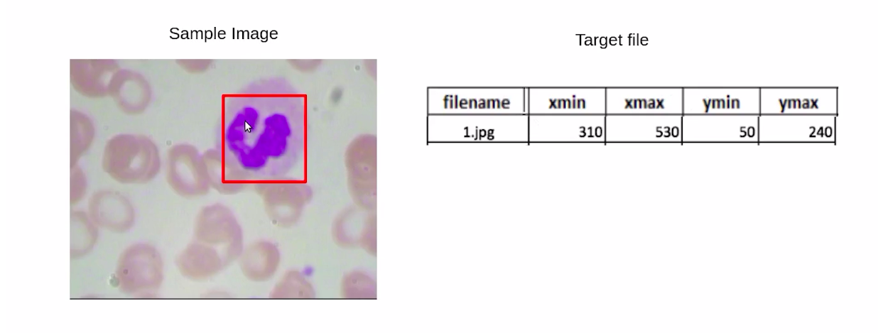
Now, for each image, we have a bounding box around the WBCs. And as you can see in this image, we have the file name as 1.jpg, and these are the bounding box coordinates for the bounding box around the WBC.

In the next section, we will cover the simplest approach or the naive approach for solving this object detection problem.

Dataset Link

Dataset link:- https://courses.analyticsvidhya.com/courses/take/Applied-Computer-Vision-using-Deep-Learning/downloads/14005079-dataset-blood-cell-detection

Naive Approach for Solving Object Detection Problem

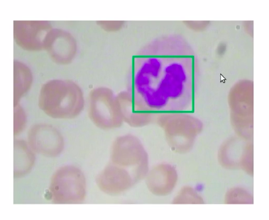
In this section, we are going to discuss a naive approach for solving the object detection problem. So let’s first understand the task, we have to detect WBCs in the image of blood cells, so you can see that below image.

Source: https://courses.analyticsvidhya.com/courses/take/Applied-Computer-Vision-using-Deep-Learning/lessons/13915284-naive-approach-one

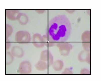
Now, the simplest way would be that divide the images into multiple patches, so for this image, have divided the image into four patches.

Source: https://courses.analyticsvidhya.com/courses/take/Applied-Computer-Vision-using-Deep-Learning/lessons/13915284-naive-approach-one

We classify each of these patches, so the first patch has no WBC the second patch has a WBC, similarly the third and fourth do not have any WBC.

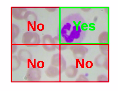
We are already familiar with the classification process and how to build the classification algorithms. So we can easily classify each of these individual patches as yes and no for representing WBC’s.

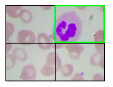
Now, in the below image the patch (a green box) which has a WBC, can be represented as the bounding box, so in this case, we’ll take the coordinates of this patch take this coordinates-value, and return that as the bounding box for WBCs.

Now in order to implement this approach, we’ll first need to prepare our training data. Now one question might be, why do we need to prepare the training data at all? we already have the images and the bounding boxes along with these images.

Well, if you remember, we have our training data in the following format where we have our WBC bounding box and the bounding box coordinates.

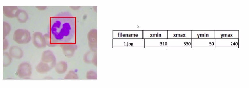
Source: https://courses.analyticsvidhya.com/courses/take/Applied-Computer-Vision-using-Deep-Learning/lessons/13915284-naive-approach-one

Now, note that we have these bounding box coordinates for the complete image, but we are going to divide this image into four patches. So we’ll need the bounding box coordinates for all of those four patches.  So our next question is how do we do that?

we have to define a new training data where we have the file name as you can see below image. We have the different patches and for each of these patches, we have Xmin, Xmax, Ymin, and Ymax values which denote the coordinates of these patches, and finally, our target variable which is WBC.  IS a WBC present in the image or not?

Now in this case it would become a simple classification problem. So for each image, we’ll divide it into four different patches and create the bounding box coordinates for each of these patches.

Now the next question is how do we create these bounding box coordinates? So it’s really simple.

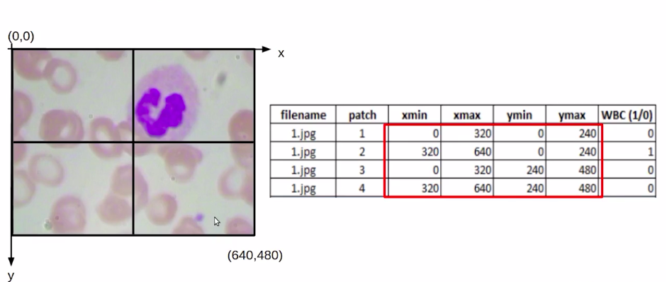
Consider this that we have an image of size (640*480). So this origin would be (0,0). The above image has x and y-axis, and here we would have the coordinate value as (640, 480).

Now, if we find out the midpoint it would be (320,240). Once we have these values, we can easily find out the coordinates for each of these patches. So for the first patch, our Xmin and Ymin would be (0,0) and Xmax, Ymax would be (320,240).

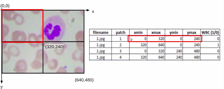
Similarly, we can find it out for the second, third, and fourth patches. Once we have the coordinate values or the bounding box values for each of these patches. The next task is to identify if there is a WBC within this patch or not.

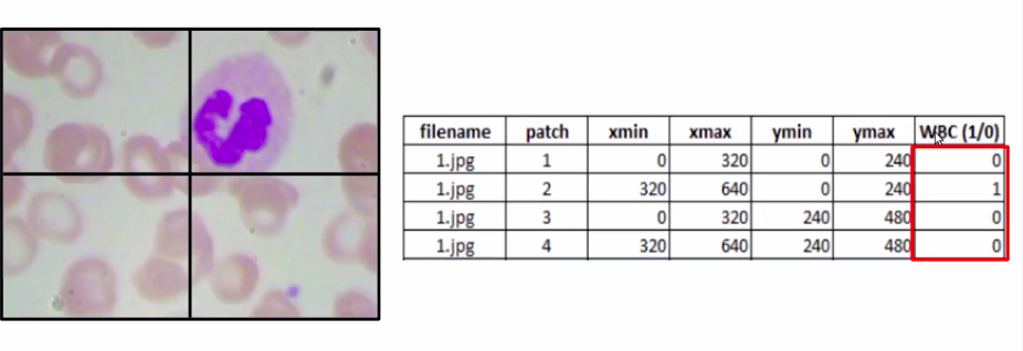
Here we can clearly see that patch 2 has a WBC while other patches do not, but we cannot manually label it for each of the images on each of the patches in the data set.

Now in the next section, we are going to implement the naive approach.

Steps to Implement Naive Approach

# Importing Required Libraries
import numpy as np
import pandas as pd
import matplotlib.pyplot as plt
%matplotlib inline
import os
from PIL import Image
from skimage.transform import resize
import torch
from torch import nn

Now we will fix a random seed value.

# Fixing a random seed values to stop potential randomness
seed = 42
rng = np.random.RandomState(seed)

here we’ll mount the drive since the data set is stored on the drive.

# mount the drive
from google.colab import drive
drive.mount('/content/drive')

Now since the data on the drive is available in the zip format. We’ll have to unzip this data and here we are going to unzip the data. So we can see that all the images are loaded and are stored in a folder called images. At the end of this folder, we have a CSV file which is trained.csv.

# unzip the dataset from drive
!unzip /content/drive/My Drive/train_zedkk38.zip

2 Data Exploration

So let us read the CSV file and find out what is the information stored in this ‘train.csv’ file.

## Reading target file
data = pd.read_csv('train.csv')
data.shape

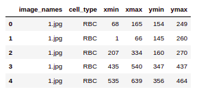
So here we are printing the first few rows of the CSV file. We can see that the file has image_names along with the cell_type which will denote RBC or WBC and so on. Finally the bounding box coordinates for this particular object in this particular image.

data.head()

So if we check the value counts for the RBC, WBC, and platelets. we’ll see that RBCs have the maximum value count followed by WBCs and platelets.

data.cell_type.value_counts()

Source: Author

Now for simplicity, we are going to only consider the WBC’s here. Hence we have selected the data with only WBC’s. So now you can see we have image_names and only cell_type WBC against these images. Also, we have our bounding box coordinates.

(data.loc[data['cell_type'] =='WBC']).head()

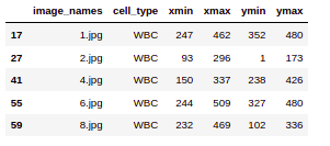
Let’s look at a few images from the original data set and the shape of these images. So we can see that the shape of these images is (480,640,3). So this is an RGB image with three channels and this is the first image in the data set.

image = plt.imread('images/' + '1.jpg')
print(image.shape)
plt.imshow(image)

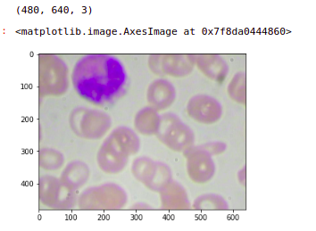
Now the next step is to create patches out of this image. So we are going to learn how to divide this image into four patches. Now we know that the image is of the shape (640, 480). hence this middle point will be (320,240) and the center is (0, 0).

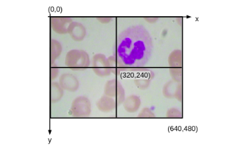
So we have the coordinates for all of these patches in the image and here we are going to make use of these coordinates and create the patches. So our format of these coordinates will be Ymin, Ymax, Xmin, and Xmax. So here we have our (Ymin, Ymax) is ( 0, 240) and (Xmin, Xmax) is (0 ,320). So this basically indicates the first patch. Similarly, we have image_2,image_3, image_4 for the subsequent second third, and fourth patches. So this is a process we can create patches from the image.

# creating 4 patches from the image
# format ymin, ymax, xmin, xmax
image_1 = image[0:240, 0:320, :]
image_2 = image[0:240, 320:640, :]
image_3 = image[240:480, 0:320, :]
image_4 = image[240:480, 320:640, :]

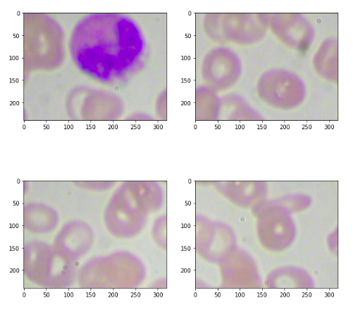
Now we need to assign a target value for these patches. So in order to do that we calculate the intersection over union where we have to find out the intersection area and the union area.

Source: Author

So intersection area is simply this particular rectangle, to find out the area we need to find out the Xmin, Xmax, and Ymin, Ymax coordinates for this rectangle.

def iou(box1, box2):
    Irect_xmin, Irect_ymin = max(box1[0],box2[0]), max(box1[2],box2[2])
    Irect_xmax, Irect_ymax = min(box1[1],box2[1]), min(box1[3],box2[3])
    if Irect_xmax < Irect_xmin or Irect_ymax < Irect_ymin:
        target = inter_area = 0
    else: 
      inter_area = np.abs((Irect_xmax - Irect_xmin) * (Irect_ymax - Irect_ymin))
      box1_area = (box1[1]-box1[0])*(box1[3]-box1[2])
      box2_area = (box2[1]-box2[0])*(box2[3]-box2[2])
      union_area = box1_area+box2_area-inter_area
      iou = inter_area/union_area
      target = int(iou > 0.1)
    return target

We have our original bounding box coordinates from the train CSV file. When I used as input these two values to the “iou” function that we defined the target comes out to be 1. You can try with different patches also based on that you will get target value.

box1= [320, 640, 0, 240]
box2= [93,    296, 1, 173]
iou(box1, box2)

The output is 0. Now the next step is to prepare the dataset.

3 Preparing Dataset for Naive Approach

We have considered and explored only a single image from the dataset. So let us perform these steps for all the images in the data set. so first of all here is the complete data that we have.

data.head()

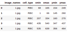
Source: Author

Now, We are converting these cell types as RBC is zero, WBC is one, and platelets are two.

data['cell_type'] = data['cell_type'].replace({'RBC': 0, 'WBC': 1, 'Platelets': 2})

Now we have to select the images which have only a single WBC.

So first of all we are creating a copy of the dataset and then keeping only WBCs and removing any image which has more than one WBC.

## keep only Single WBCs
data_wbc = data.loc[data.cell_type == 1].copy()
data_wbc = data_wbc.drop_duplicates(subset=['image_names', 'cell_type'], keep=False)

So now we have selected the images. We are going to set the patch coordinates based on our input image sizes. We are reading the images one by one and storing the bounding box coordinates of the WBC for this particular image. We are extracting the patches out of this image using the patch coordinates that we have defined here.

And then we are finding out the target value for each of these patches using the IoU function that we have defined. Finally, here we are resizing the patches to the standard size of (224, 224, 3). Here we are creating our final input data and the target data for each of these patches.

# create empty lists
X = []
Y = []
# set patch co-ordinates
patch_1_coordinates = [0, 320, 0, 240]
patch_2_coordinates = [320, 640, 0, 240]
patch_3_coordinates = [0, 320, 240, 480]
patch_4_coordinates = [320, 640, 240, 480]
for idx, row in data_wbc.iterrows():
    # read image
    image = plt.imread('images/' + row.image_names)
    bb_coordinates = [row.xmin, row.xmax, row.ymin, row.ymax]
    # extract patches
    patch_1 = image[patch_1_coordinates[2]:patch_1_coordinates[3],
                             patch_1_coordinates[0]:patch_1_coordinates[1], :]
    patch_2 = image[patch_2_coordinates[2]:patch_2_coordinates[3], 
                               patch_2_coordinates[0]:patch_2_coordinates[1], :]
    patch_3 = image[patch_3_coordinates[2]:patch_3_coordinates[3], 
                            patch_3_coordinates[0]:patch_3_coordinates[1], :]
    patch_4 = image[patch_4_coordinates[2]:patch_4_coordinates[3], 
                            patch_4_coordinates[0]:patch_4_coordinates[1], :]
    # set default values
    target_1 = target_2 = target_3 = target_4 = inter_area = 0
    # figure out if the patch contains the object
    ## for patch_1
    target_1 = iou(patch_1_coordinates, bb_coordinates )
    ## for patch_2
    target_2 = iou(patch_2_coordinates, bb_coordinates)
    ## for patch_3
    target_3 = iou(patch_3_coordinates, bb_coordinates)
    ## for patch_4
    target_4 = iou(patch_4_coordinates, bb_coordinates)
    # resize the patches
    patch_1 = resize(patch_1, (224, 224, 3), preserve_range=True)
    patch_2 = resize(patch_2, (224, 224, 3), preserve_range=True)
    patch_3 = resize(patch_3, (224, 224, 3), preserve_range=True)
    patch_4 = resize(patch_4, (224, 224, 3), preserve_range=True)
    # create final input data
    X.extend([patch_1, patch_2, patch_3, patch_4])
    # create target data
    Y.extend([target_1, target_2, target_3, target_4])
# convert these lists to single numpy array
X = np.array(X)
Y = np.array(Y)

Now, let’s print the shape of our original data and the new data that we have just created. So we can see that we originally had 240 images. Now we have divided these images into four parts so we have (960,224,224,3). This is the shape of the images.

# 4 patches for every image
data_wbc.shape, X.shape, Y.shape

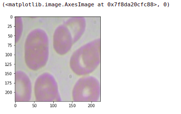
so let’s quickly look at one of these images that we have just created. So here is our original image and this is the last patch or the fourth patch for this original image. We can see that the target assigned is one.

image = plt.imread('images/' + '1.jpg')
plt.imshow(image)

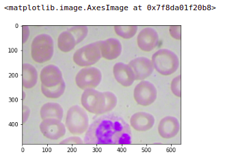
If we check any other patch, let’s say I want to check the first patch of this image so here this will put the target as zero. You will get the first patch. Similarly, you can ensure that all the images are converted into patches and the targets are assigned accordingly.

plt.imshow(X[0].astype('uint8')), Y[0]

4 Preparing Train and Validation Sets

Now that we have the dataset. we are going to prepare our training and validation sets. Now note that here we have the shape of images as (224,224,3).

# 4 patches for every image
data_wbc.shape, X.shape, Y.shape

The output is:-

((240, 6), (960, 224, 224, 3), (960,))

In PyTorch, we need to have the channels first. So we are going to move the axis that is will have the shape (3,224,224).

X = np.moveaxis(X, -1, 1) 
X.shape

The output is:-

(960, 3, 224, 224)

Now here we are normalizing the image pixel values.

X = X / X.max()

Using the train test split function we are going to create a train and validation set.

from sklearn.model_selection import train_test_split
X_train, X_valid, Y_train, Y_valid=train_test_split(X, Y, test_size=0.1, 
                                            random_state=seed)
X_train.shape, X_valid.shape, Y_train.shape, Y_valid.shape

The output of the above code is:-

((864, 3, 224, 224), (96, 3, 224, 224), (864,), (96,))

Now, we are going to convert both of our training sets and validation sets into tensors, because these are “numpy” arrays.

X_train = torch.FloatTensor(X_train)
Y_train = torch.FloatTensor(Y_train)
X_valid = torch.FloatTensor(X_valid)
Y_valid = torch.FloatTensor(Y_valid)

5 Model Building

For now, we’re going to build our model so here we have installed a library which is PyTorch model summary.

!pip install pytorch-model-summary

 

This is simply used to print the model summary in PyTorch. Now we are importing the summary function from here.

from pytorch_model_summary import summary

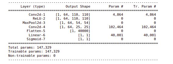
Here is the architecture that we have defined for our Naive approach. So we have defined a sequential model where we have our Conv2d layer with the input number of channels as 3 and the number of filters is 64, the size of the filters is 5 and the stride is set to 2. We have our ReLU activation function for this Conv2d layer. A pooling layer with the window size as 4 and stride 2 and then convolutional layer. Now we are flattening the output from the Conv2d layer and finally our linear layer or dense layer and sigmoid activation function.

## model architecture
model = nn.Sequential(
        nn.Conv2d(in_channels=3, out_channels=64, kernel_size=5, stride=2),  
        nn.ReLU(),  
        nn.MaxPool2d(kernel_size=4,stride=2),   
        nn.Conv2d(in_channels=64, out_channels=64, kernel_size=5, stride=2),    
        nn.Flatten(),
        nn.Linear(40000, 1),
        nn.Sigmoid()
)

So here if we print the model this will be the model architecture that we have defined.

print(model)

 

Using the summary function, we can have a look at the model summary. So this will return us the layers the output shape from each of these layers, the number of trainable parameters for each of these layers. So now our model is ready.

print(summary(model, X_train[:1]))

 

Now the model is ready for the train.

6 Train the Model

let us train this model. So we are going to define our loss and optimizer functions. We have defined binary cross-entropy as a loss and adam optimizer. And then we are transferring the model to GPU. Here we are taking batches from the input image in order to train this model.

## loss and optimizer
criterion = torch.nn.BCELoss()
optimizer = torch.optim.Adam(model.parameters(), lr=0.001)

## GPU device
if torch.cuda.is_available():
  model = model.cuda()
  criterion = criterion.cuda()

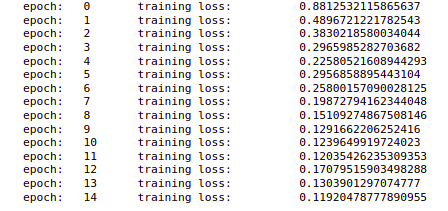
So we have taken batches from our x_train and used these batches. we are going to train this model for a total of 15 epochs. We have also set an optimizer.Zero_grad() and we are storing the outputs here.
Now we are calculating the losses and storing all the losses and performing the backward propagation and updating the parameters. Also, we are printing the loss after every epoch.
In the output, we can see that at each epoch the loss is decreasing. So the training is complete for this model.

# batch size of the model
batch_size = 32
# defining the training phase
model.train()
for epoch in range(15):
    # setting initial loss as 0
    train_loss = 0.0        
    # to randomly pick the images without replacement in batches
    permutation = torch.randperm(X_train.size()[0])
    # to keep track of training loss
    training_loss = []
    # for loop for training on batches
    for i in range(0,X_train.size()[0], batch_size):
        # taking the indices from randomly generated values
        indices = permutation[i:i+batch_size]
        # getting the images and labels for a batch
        batch_x, batch_y = X_train[indices], Y_train[indices]
        if torch.cuda.is_available():
            batch_x, batch_y = batch_x.cuda().float(), batch_y.cuda().float()
        # clearing all the accumulated gradients
        optimizer.zero_grad()
        # mini batch computation
        outputs = model(batch_x)
        # calculating the loss for a mini batch
        loss = criterion(outputs.squeeze(),batch_y)
        # storing the loss for every mini batch
        training_loss.append(loss.item())
        # calculating the gradients
        loss.backward()
        # updating the parameters
        optimizer.step()
    training_loss = np.average(training_loss)
    print('epoch: t', epoch, 't training loss: t', training_loss)

 

7 Make Predictions

Let us now use this model in order to make predictions. So here I am only taking the first five inputs from the validation set and transferring them to the Cuda.

output = model(X_valid[:5].to('cuda')).cpu().detach().numpy()

Here is the output for these first five images that we have taken. Now we can see that for the first two the output is that there is no WBC or there is a WBC.

output

This is the output:

array([[0.00641595],
       [0.01172841],
       [0.99919134],
       [0.01065345],
       [0.00520921]], dtype=float32)

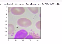
So let’s also plot the images. We can see that this is the third image, here the model says that there is a WBC and we can see that we have a WBC in this image.

plt.imshow(np.transpose(X_valid[2]))

 

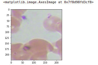
Similarly, we can check for another image, So will take the first image of the output. you can see the output image, this image was our input patch and there is no WBC in this patch.

plt.imshow(np.transpose(X_valid[1]))

 

This was a very simple method in order to make the predictions or identify the patch or portion of the image that has a WBC.

Conclusion

About the Author

Hi, I am Kajal Kumari. have completed my Master’s from IIT(ISM) Dhanbad in Computer Science & Engineering. As of now, I am working as Machine Learning Engineer in Hyderabad. Here is my Linkedin profile if you want to connect with me.

End Notes

Thanks for reading!

I hope that you have enjoyed the article. If you like it, share it with your friends also. Please feel free to comment if you have any thoughts that can improve my article writing.

If you want to read my previous blogs, you can read Previous Data Science Blog posts from here.

The media shown in this article is not owned by Analytics Vidhya and are used at the Author’s discretion.

kajal

Hi, I am Kajal Kumari. have completed my Master’s from IIT(ISM) Dhanbad in Computer Science & Engineering. As of now, I am working as Machine Learning Engineer in Hyderabad.
hope that you have enjoyed the article. If you like it, share it with your friends also. Please feel free to comment if you have any thoughts that can improve my article writing.

If you want to read my previous blogs, you can read Previous Data Science Blog posts here. Connect with me