Introduction
Computer vision is a field of A.I. that deals with deriving meaningful information from images. Since 2012 after convolutional neural networks(CNN) were introduced, we moved away from handcrafted features to an end-to-end approach using deep neural networks. These are easy to develop i.e. they require minimum domain expertise and they tend to perform better for most of the vision-related tasks. But they come with a set of problems that most neural networks model have. They need data, lots and lots of annotated data for training.
Take an example of the task of classifying an image as a car or a truck. We need to show lots of images of both classes i.e. cars and trucks and then we hope that model learns distinguishing patterns. But nowadays lots of images of futuristic-looking concept cars are popping up. If we don’t have lots of images of such cars in our training data labeled as ‘concept cars’ our model might not be able to distinguish them from regular cars during inference. This problem is much more severe in the medical domain where collecting gold standard data for training is challenging. And a general-purpose model trained on the imagenet dataset is completely useless in the medical domain.
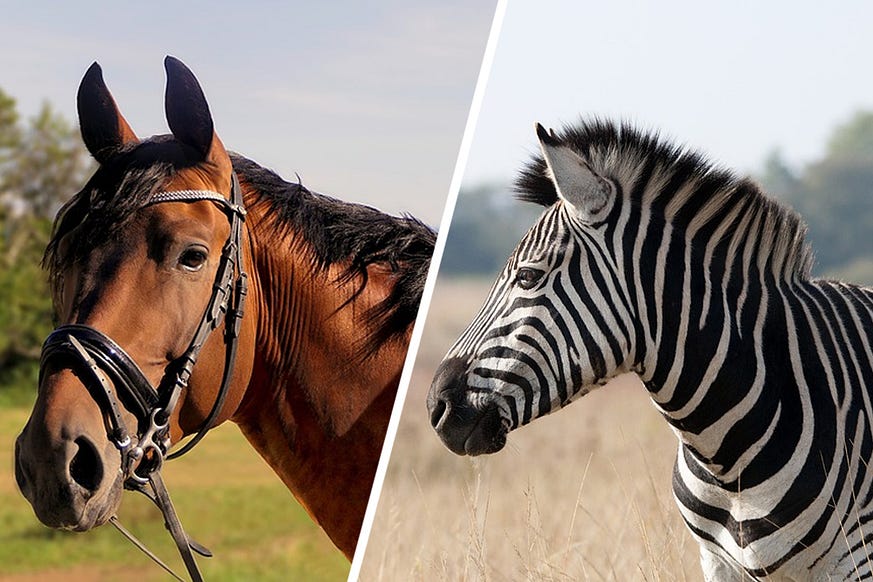
Let’s see how a human might do it. Suppose a person knows what a horse looks like. And give that person the info that ‘A zebra is a horse with black and white striped skin’. Then there is a high chance that a person can identify a zebra even though that person had no prior idea of what a zebra is. Zero-shot learning is an approach in machine learning that takes inspiration from this.
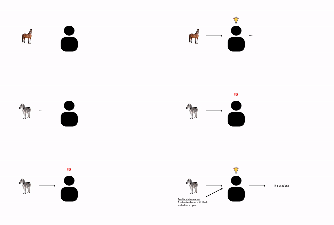
In a zero-shot learning approach we have data in the following manner:
- Seen classes: Classes with labels available for training.
- Unseen classes: Classes that occur only in the test set or during inference. Not present during training.
- Auxiliary information: Information about both seen and unseen class labels during training time.
Types of Zero-Shot Learning
Based on the data available during inference zero-shot learning can be classified into two types
- Conventional zero-shot learning: If during test time we only expect images from unseen classes.
- Generalized zero-shot learning: If during testing phase images from both seen and unseen class can be present. For most practical use cases, we will be using this mode of zero-shot learning.
Approach 1
Here the idea is to represent the input image in the same vector space as the auxiliary information. To learn the hidden representations an encoder is used that tries to map a given image to its auxiliary information. The auxiliary information is used as gold data using which our encoder learns.
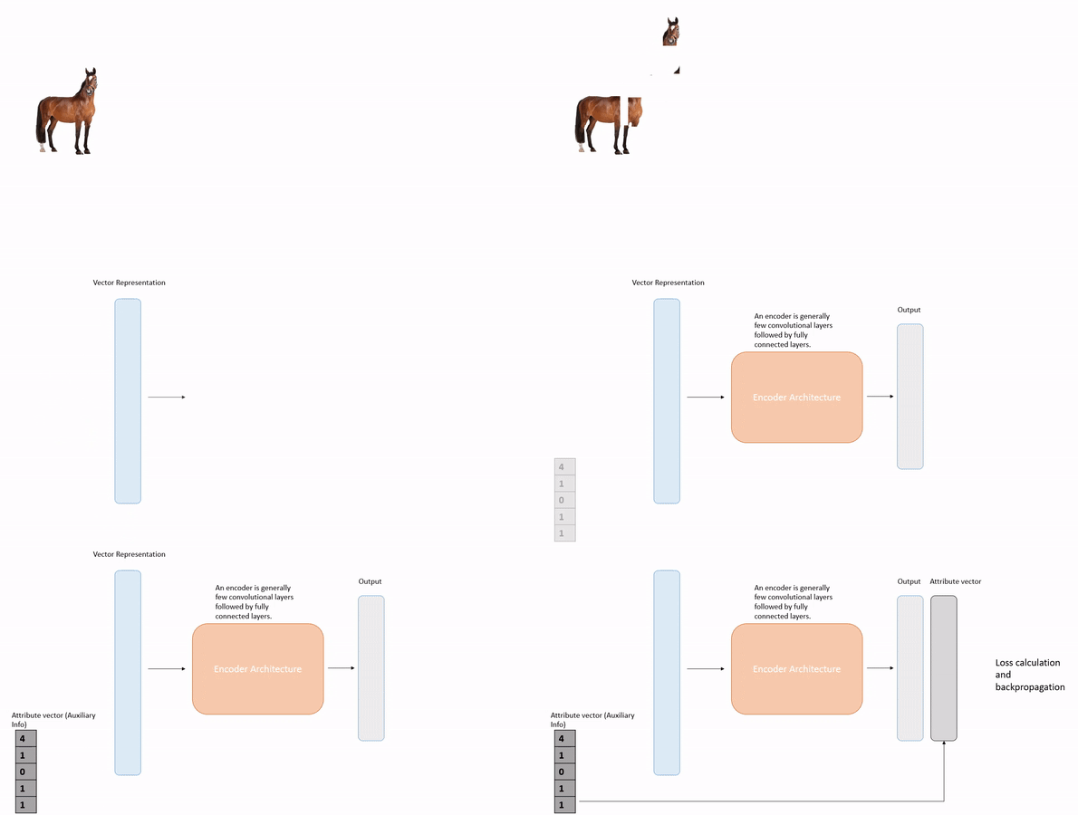
Source: Author
The attribute vector shown above is just for understanding purposes. Nowadays with the advent of transformer-based models, we can generate many sophisticated word embedding vectors.
That is the training phase. In the testing phase, we will use the trained encoder and when an image comes we will pass it through the encoder to generate an output vector. Then we can find the most similar auxiliary vector to our output. That will be our prediction.
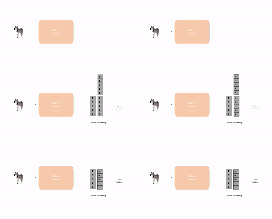
Although theoretically this approach seems nice but it suffers from a lot of inherent problems. Since the encoder will be trained on seen class images there is a chance that it might not be able to bridge the gap and generalize for the unseen classes. It might be biased towards seen class.
Another problem is semantic loss. If the model is trained mostly on four-legged animals then the feature number of legs might become useless. But while testing if a two-legged animal comes since the model chose to make the number of legs feature irrelevant it might not be able to classify properly during the test phase.
Finally, we also face the problem of hubness. When we pass an image through the encoder we are in a way reducing its dimensionality. This process reduces the spread of the data and tends to form clusters that were not present in higher dimensions. When we try to find similar vectors this tends to give incorrect results.
Approach 2
This is another approach that addresses a few problems of the previous approach.
One major problem of this approach is that there were no unseen class images while training the encoder. Here we will use a generative network to generate unseen class images for training using the auxiliary information.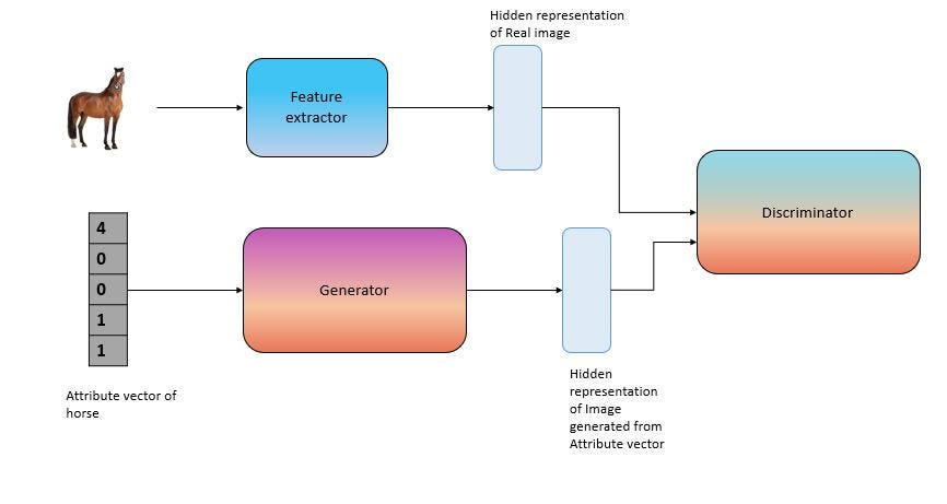
Source: Author
Here we will try to use the auxiliary information to generate an image of the corresponding class. Then we will also have the actual image. The task of the discriminator will be to differentiate between real and generated images. Initially, the generator will be very weak so the discriminator will easily identify the difference. But as we keep on training at a point it will become very difficult for the discriminator to identify the difference. Then we will stop the training and we will have a trained generator. We can use this trained generator to generate images from unseen classes for training.
To evaluate a zero-shot recognition model top -1 accuracy metric is generally used. This metric is similar to accuracy but for zero-shot, we take the average accuracy of both the seen and unseen classes. We want both their accuracy to be high for this reason Harmonic mean of the accuracy of both classes is selected as a metric. The value we get as a harmonic mean will be close to the minimum of both accuracy values.


Code
For understanding the working of zero-shot learning we can use the hugging face library. We have a predefined zero-shot classification pipeline where we can pass ‘zero-shot classification’ to initialize the pipeline.

Once the pipeline is initialized we can pass the text sequence and possible candidate labels to classify.

As you can see ‘gymnasium’ has the highest score.
Conclusion
We have seen how the zero-shot learning approach alleviates the dependency on training data. This can be thought of as a transfer learning approach where we try to transfer information from target classes.
Read more articles on Machine Learning on our blog.
References
- https://www.kdnuggets.com/2021/04/zero-shot-learning.html
- https://cetinsamet.medium.com/zero-shot-learning-53080995d45f
- https://arxiv.org/pdf/1707.00600v4.pdf
About the Author
Please feel free to connect with me:
If any queries please feel free to ask in the comments.
Have a nice day!
The media shown in this article is not owned by Analytics Vidhya and are used at the Author’s discretion.


