Industrial Application of NLP: Task I

This article was published as a part of the Data Science Blogathon.

An end-to-end Guide on Consumer Complaint Segregation using NLP

Hey Folks!

In this article, we are going to solve a real Business Problem that is Consumer Complaint Segregation using basic concepts of NLP in a very detailed manner.

I believe that you are already comfortable with the concepts of natural language processing basics like feature extraction, working with raw data, and comfortable with model training on textual data.

I have already written a series of detailed articles on NLP starting from zero, so if you are not comfortable with the basics of NLP you can refer to my articles.

Table of Content

• Introduction & Goal
• loading the data
• Feature Engineering & Feature Extraction
• Exploratory Data Analysis (EDA)
• Text Preprocessing
• Training Multi-Classification Model
• Recall, Precision, F1-score
• Predictions

Introduction

Financial Protection Bureau is an organization that sends thousands of consumers’ complaints about financial services (mortgage, student loans, etc.) and products ( ie. credit cards, debit cards) for some response.

Complaints need to be segregated and deliver to the concerning department, this increases the response time of complaints since we are reducing the human intervention to classify the complaint category.

So we need to build a model that reads the complaint and can tell us the concerning department like complaints related to the mortgage must be forwarded to the mortgage department and credit card complaints to be forwarded to the banking products department.

Goal

The Goal of this Project is to segregate the complaint into their concerning product or category department.

Since the complaint can be more than two hence it will be a multi-class classification and it can be solved by using NLP and machine learning algorithms.

By using the Machine learning model we can easily classify the complaint hence we are reducing the human intervention to classify the complaint and reducing the response time of complaints.

Note: Text classification is an example of supervised machine learning because we are working on labelled data for training and testing purpose.

Let us start working on this Project.

1. Loading & Understanding the Dataset

We are going to work on the Consumer Finance Complaints Dataset provided by the Bureau of Consumer Financial Protection.

You can download the dataset using this link or you can create a cloud Notebook and work instantly.

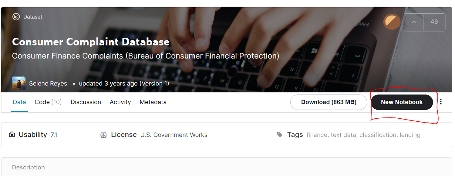
• Loading the dataset into Pandas data frame

import pandas as pd
import numpy as np
df = pd.read_csv("../input/consumer-complaint-database/rows.csv", low_memory = False)
df.head()

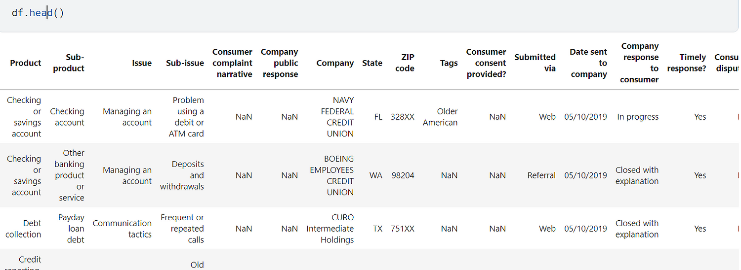
This dataset contains so many columns but we need to focus on only two columns [Product, Consumer complaint narrative].

• Product → Category of Complaint
• Consumer complaint narrative → Consumer’s Complaint text

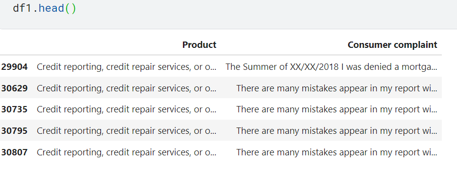
df1 = df[['Product', 'Consumer complaint narrative']]
df1.columns = ['Product', 'Consumer complaint']

We have renamed the “consumer complaint narrative” to “Consumer complaint” and kept in a data frame df1 .

• Filtering the Complaints with No text (False Complaint )

In the dataset there are many complaints with no text body, these are false complaints we need to filter such complaints out.

df1 = df1[df1['Consumer complaint'].isna() != True]

2. Feature Engineering

Under Feature Engineering we do some data manipulation in order to train the model efficiently and get a better insight into the data.

pd.DataFrame(df1.Product.unique()).values

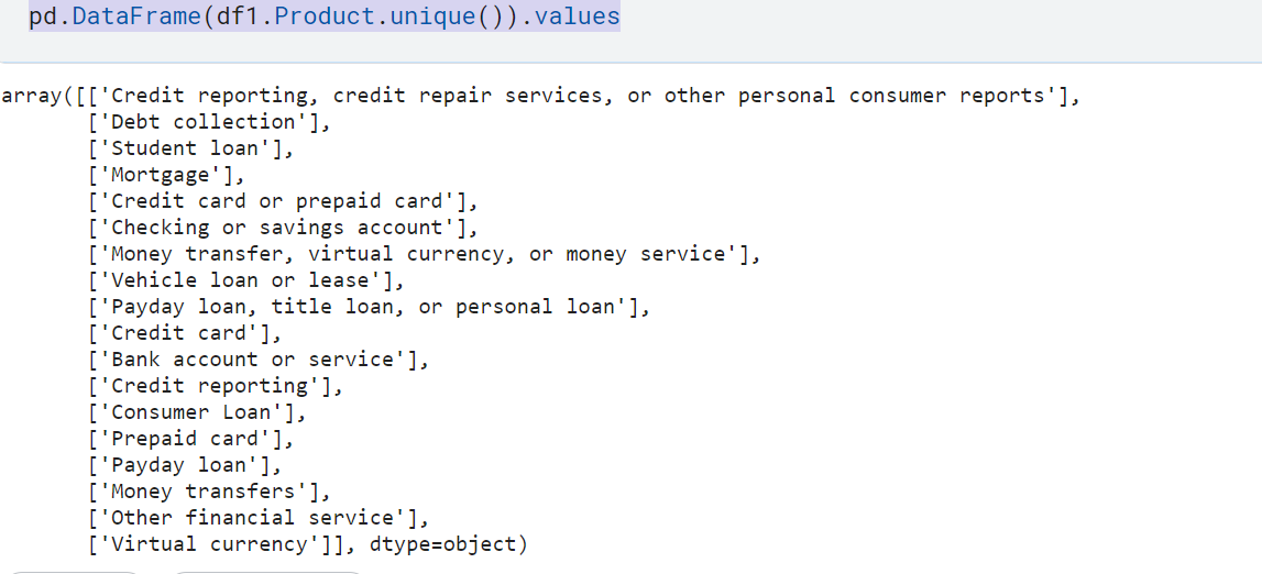
In our dataset, we have 18 different complaints categories, some of the complaint categories are interrelated. for instance “Credit card of the prepaid card” and “Prepaid Card”, “Credit card” are so related.

Hence we need to rename the categories in order to merge related categories.

• Renaming the Categories

# Renaming categories by using 
df1.replace({'Product': 
             { 
              'Credit reporting': 'Repair or Credit reporting',
             'Credit card': 'Credit card or prepaid card',
             'Prepaid card': 'Credit card or prepaid card',
            'credit repair services,Credit reporting , or other personal consumer reports': 
            'Repair or Credit reporting',
             'Money transfer': 'Money transfer, virtual currency, or money service',
            'Payday loan': 'title loan,Payday ,Personal loan',
             'Virtual currency': 'Money transfer, virtual currency, or money service'}}, 
            inplace= True)

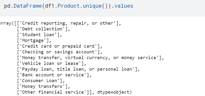
After renaming we have only 13 categories / Products to classify.

Note: The Dataset we are working on is too big . it contains 1.2 millions of rows , hence training on a big data will be so time consuming , so we will take only sample of 10000 rows for our training in order to save time.

df2 = df1.sample(10000, random_state=1).copy()

here df2 is the dataset we will further work on and it contains 10000 rows and 2 columns

• so far we have the dataset in text and we need to convert the complaint text and category into some number

Converting the Categories (Product) into numbers

df2['category_id'] = df2['Product'].factorize()[0]

We have added a new column “category_id” and it will contain the category number.

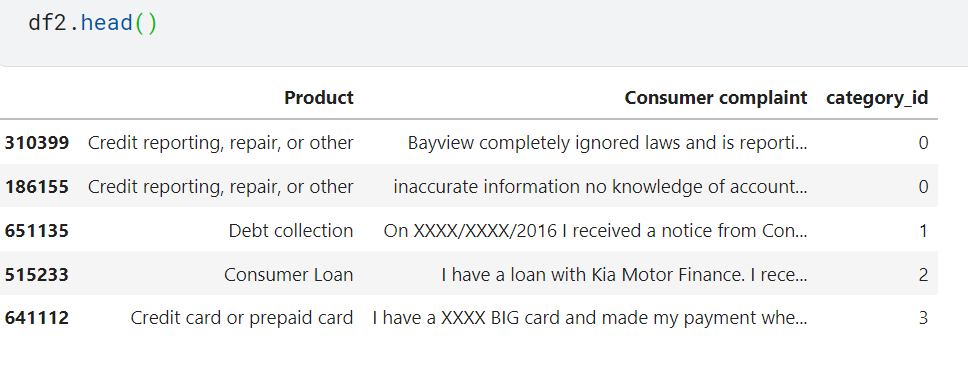
• As you see we have converted the category label into category_id we also need data to convert category_id back to the category label at the time of prediction. For this purpose, we will create a dictionary.

category_id = df2[['Product', 'category_id']].drop_duplicates()
id_2_category = dict(category_id[['category_id', 'Product']].values)

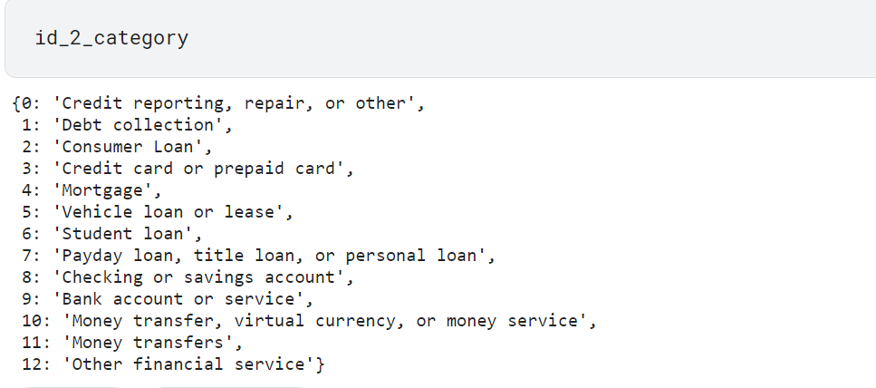
we will use id_2_category dictionary for converting class_id to class_lable.

3. Performing EDA

Under EDA we explore our data, we plot charts to understand the relation and various insights of the data.

Plotting the Product/Categories vs Number of Complaints

import matplotlib.pyplot as plt
import seaborn as sns
fig = plt.figure(figsize=(8,6))
colors = ['grey','grey','grey','grey','grey','grey','grey','grey','grey',
    'grey','darkblue','darkblue','darkblue']
df2.groupby('Product')['Consumer complaint'].count().sort_values().plot.barh(
    ylim=0, color=colors, title= 'NUMBER OF COMPLAINTS IN EACH PRODUCT CATEGORYn')
plt.xlabel('Number of ocurrences', fontsize = 10)

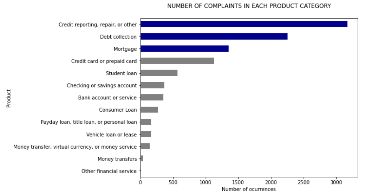
You can Possibly see that “credit reporting, repair and other “ have the maximum supporting records and “Other financial Services” have very few records. This shows some Possible data imbalance and this can be fixed by sampling equal records from each category/Product.

4. Feature Engineering

Now we need to convert the Complaint text into some vectors since the machine can’t understand the textual data. This process is called Feature Extraction.

We are going to use tf-idf Vectorizer ( Inverse Document Frequency ) for feature extraction. If you are not comfortable with Feature Engineering prefer my article.

TFIDF evaluated how important a word is to its document in a collection or group of documents.

Note: After removing punctuation, lower caseing the words we can proceed to the feature extraction step. TFIDF vectorizer can handle the stopwords on its own.

Term Frequency: This tells how often a given word occurs within a document.

Inverse Document Frequency: It is the opposite of the Term Frequency. If a given word appears many times among the documents it will have a low IDF score.

from sklearn.feature_extraction.text import TfidfVectorizer
tfidf = TfidfVectorizer(sublinear_tf=True, min_df=5,
                        ngram_range=(1, 2), 
                        stop_words='english')

# Vectorization
features = tfidf.fit_transform(df2['Consumer complaint']).toarray()
labels = df2.category_id

• min_df: it removes those words from the vocabulary which has appeared less than ‘min_df’ number of files.
• sublinear_tf = TrueScale the term frequency on a logarithmic scale.
• stop_words: removes the stopwords of mentioned language.
• ngram_range =(1, 2) Unigram and bigram both will be considered
• max_df: It removes those words from the vocabulary which have appeared more than ‘maxdf’

Splitting the Dataset

Splitting the dataset into training and testing partitions. 75% of the records will be used for training and the rest will be used for testing purposes.

from sklearn.model_selection import train_test_split
X_train, X_test, y_train, y_test = train_test_split(features, labels, 
                                                    test_size=0.25,
                                                    random_state = 0)

5. Model Training

We are going to use LinearSVC hence it performed well you can try other models as well and check their performance.

from sklearn.svm import LinearSVC
model = LinearSVC()
model.fit(X_train, y_train)

6. Evaluation and Testing

In order to see how our model performs we will use sklearn’s metrics class. We will use a Classification report and confusion matrix.

from sklearn import metrics
from sklearn.metrics import classification_report
# Classification report
y_pred = model.predict(X_test)
print(metrics.classification_report(y_test, y_pred, 
                                    target_names= df2['Product'].unique()))

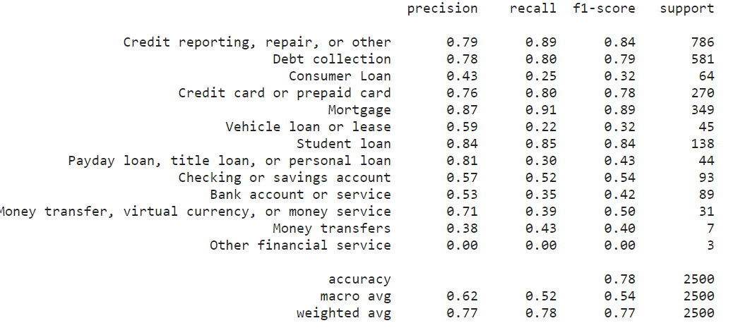
As you observe classes having more support ( data rows) are having better f1-score. this is happening because those classes are trained on more data. To fix this issue we should balance the data, as we have discussed already.

classes like ‘Mortgage’, ‘Student loan ‘Credit reporting, repair, or other’ can be classified with more precision.

Plotting Confusion Matrix

import seaborn as sns
sns.set()
from sklearn.metrics import confusion_matrix
conf_mat = confusion_matrix(y_test, y_pred)
fig, ax = plt.subplots(figsize=(8,8))
sns.heatmap(conf_mat, annot=True, cmap="Blues", fmt='d',
            xticklabels=category_id.Product.values, 
            yticklabels=category_id.Product.values)
plt.ylabel('Actual')
plt.xlabel('Predicted')
plt.title("CONFUSION MATRIX - LinearSVCn", size=16);

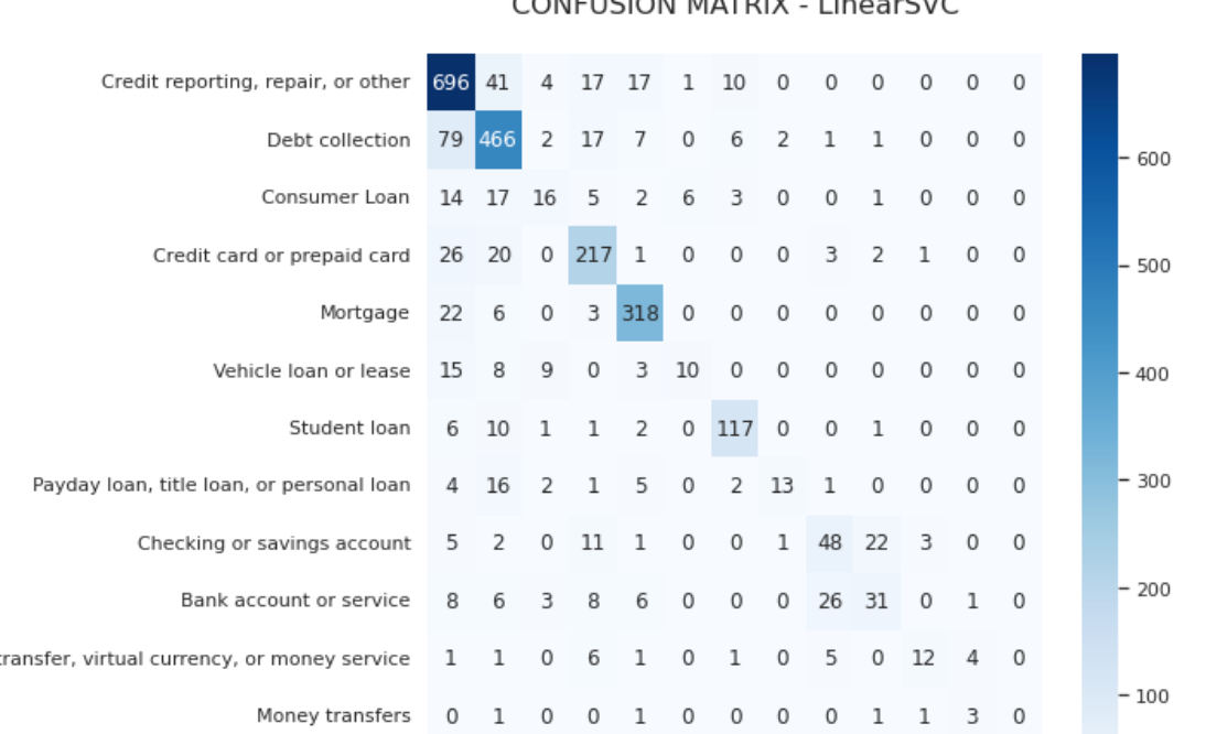
It is clearly observable that Credit card reporting and data collection classes have more precision than others do.

7. Prediction

It’s time to try our model for some prediction. we will pass a complaint text and our model will classify according to its complaint class.

complain = """I have been enrolled back in 2019 to Indian University. Few days ago , i have been harassed by 
Navient. I have already faxed the paperwork providing them with everything they wanted. And still getting 
phone calls for payments. Furthermore, Navient is now reporting to the credit bureaus that I am late for the payment. At this point, 
Navient needs take their act together to avoid me taking further steps"""

We can’t pass text directly to the trained model for prediction we need to use our fitted vectorizer for feature extraction and then only we will pass our features for prediction.

complaint_id = (model.predict(tfidf.transform([complain])))
print("complain", id_2_category[complaint_id[0]])

output:

complain student loan

It’s clearly visible that our model has predicted accurately.

Conclusion

In this article we have Solved a Business Problem using NLP, we used various concepts like data cleaning, EDA, feature extraction, feature engineering, and successfully build our model for segregation of complaints types.

Further, you can try different models like BERT, LSTM for classification, you can also give a try to word embedding since word embedding holds an upper hand compared to TFIDF Vectorizer.

In the next article, we will cover Text summarization for subject notes with simple implementation with Python.

Read more articles on NLP on our website

If you have any suggestions or questions for me feel free to hit me on my Linkedin.

Thanks for reading !!

The media shown in this article is not owned by Analytics Vidhya and are used at the Author’s discretion.

Abhishek Jaiswal

A data enthusiast exploring the leading technologies related to the data