Logistic Regression using Python and Excel

Introduction

Will tomorrow be a sunny day? What are the chances that a student will get into that dream university? These and many more real-world “decision” scenarios need a standard mechanism. Step in Logistic Regression may be stated simply as an estimation of the probability of an event occurring. In the next few minutes, we shall understand Logistic Regression from A-to-Z. We will first implement it using MS Excel and then Python (using packages like sklearn and statsmodel) to obtain regression coefficients. This should help reinforce and ensure a holistic understanding of the concept. We conclude by interpreting the chosen regression coefficient regarding the odds ratio. Of course, we will need a dataset to work with, so let’s get it out of the way first and then focus on the subject matter.

This article was published as a part of the Data Science Blogathon.

About the Dataset

I have created a dummy dataset for this implementation, much smaller than anything you encounter in the wild. Our dataset deals with Common Entrance Test (CET) scores and determines whether a student will succeed in getting university admission. For this, the dataset has one ‘independent’ or ‘predictor’ variable: the Common Entrance Test (CET) score and a ‘dependent’ or ‘response’ variable (whether the student makes the cut or not, whether they get in or not). Our problem statement is to predict whether students can get into a university given their CET score.

What is Logistic Regression?

In logistic regression, the target variable differs from linear regression as it’s discrete rather than continuous. This distinction makes logistic regression well-suited for tackling classification problems in supervised machine-learning models. The output of a logistic function provides an estimate of the probability of a specific event happening, with probabilities always falling within the range of 0 to 1. Setting a random state can be advantageous when implementing logistic regression algorithms in machine learning models to ensure reproducibility and consistency in results.

Understanding the odds ratio

If the Probability of a particular event occurring is p, then the probability of that event not occurring is (1-p). The ratio of p to (1-p) is called the Odds, as follows-

In simple linear regression, the model to estimate the continuous response variable y as a linear function of the explanatory variable x as follows:

However, when the response variable is discrete, such as definite, with values of 1 or 0 (True or False, Success or Failure), estimation is conducted based on the probability of success. This scenario commonly arises in binary classification tasks. Logistic regression, a popular method for binary classification, models the estimate of probability p in terms of the predictor or explanatory variables x. The natural log of odds, also known as the logit function, is employed for this transformation. For a single predictor variable, the transformation equation is given as follows:

Estimate of Probability can also be written in terms of sigmoid function as:

Using MS Excel for Logistic Regression

Watch the video explaining how to obtain logistic regression coefficients in MS Excel:

Logistic Regression with Python

To do this, we shall first explore our dataset step-by-step using Exploratory Data Analysis (EDA), then implement logistic regression, and finally interpret the odds..

Step 1: Import required libraries

In this analysis, we use the built-in scikit-learn packages to split data into training and test sets and implement logistic regression. Next, we employ the predict_proba function to generate probability estimates for the outcomes. We also use the confusion_matrix and accuracy_score functions to evaluate the model’s performance. Visualizations play a crucial role in our analysis, with a heatmap from the Seaborn package employed to visualize the confusion matrix. Additionally, we utilize Boxplot from Seaborn to detect outliers within the dataset.

#import the relevant libraries
import numpy as np
import matplotlib.pyplot as plt
import pandas as pd
import seaborn as sns
from sklearn.linear_model import LogisticRegression
from sklearn.model_selection import train_test_split
from sklearn.metrics import confusion_matrix, accuracy_score
%matplotlib inline
import warnings #to remove the warnings
warnings.filterwarnings('ignore')

Step 2: Load, visualize and explore the dataset

df= pd.read_csv('/content/CET_logistics_1.csv') #read the dataset
#Explore the dataset
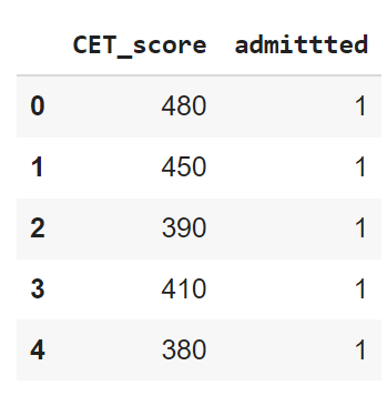
df.head()
df.describe() #To know more about the dataset
 

Output:

Step 3: Clean the data set

The output of the described method shows that the CET_score column doesn’t contain any zeros. However, to ensure the integrity of our data, we also need to assess the presence of null entries across all columns in the data frame. This evaluation is crucial for obtaining accurate performance metrics, including the f1-score, which relies on reliable and complete data.

#Check for null entries
print("Number of null values in the data set are - ",df.isnull().values.any().sum())

It is understood that there are no null values in the dataset. However, it is observed that the target column ‘admitted’ have non-numerical values ‘Yes’ an To ad’ To address this, preprocessing steps are employed using the tools provided by the sklearn library. ‘Yes’ and ‘No’ are replaced with numbers 1 and 0 respectively, facilitating further analysis.”

#Replace yes and no entries in target to 1 and 0 repsectively
df=df.replace({'admittted':{'Yes':1, 'No':0}})

Output:

Step 4: Deal with the outliers

The following code is implemented to check any outliers in the predictor variables.

#Boxplot to visualize outliers in-depth column
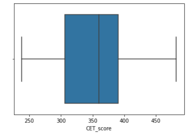
sns.boxplot(df['CET_score'])

Output:

The boxplot shows that there are no outliers below the 25th percentile and above the 75th percentile, indicating a balanced distribution. Hence, there is no requirement to eliminate any outliers. Nevertheless, should the need arise to address outliers, one could employ the following function, considering the importance of monitoring AUC and iteration performance throughout the process.

#Function to find the upper and lower limits to identify and remover outliers
def interQuartile(x):
  percentile25= x.quantile(0.25)
  percentile75=x.quantile(0.75)
  iqr=percentile75-percentile25
  upperLimit= percentile75+1.5*iqr
  lowerLimit= percentile25-1.5*iqr
  return upperLimit, lowerLimit
"""
To find the upper and lower limit CET_score column and 
check if any values are beyond these limits
"""
upper,lower= interQuartile(df['CET_score'])
print("Lower and upper limit calculated are -", upper, lower)

It is seen that the lower and upper limits beyond which the data point will be considered outliers are 181.25 and 515.25. Using the code below, it could be found if there are any outliers beyond the upper and lower range.

#To print the number of datapoints below and above these limits
 

print("Number of entries below the lower limit are ", (df['CET_score'] < lower).sum())
print("Number of entries above the upper limit are ", (df['CET_score'] > upper).sum())

Step 5: Define dependent and independent variables and then split the data into a training set and testing set.

In this step, the independent and dependent variables are first defined, and then the data set is split into training and testing data using a ratio of 80-20. This implementation also involves importing necessary modules from sklearn for tasks like plotting the ROC curve.

# Define the independent and dependent variables 
y= df['admittted'] 
#dependent variable is Decision 
x= df.drop(['admittted'], axis=1) 
# splitting the data 
x_train, x_test, y_train, y_test = train_test_split(x,y, test_size= 0.2)

Step 6: Fit a logistic regression model using sklearn

In this step, we create a logistic regression classifier and fit the model using the training data to obtain the regression coefficients. Additionally, we import the necessary functionality from the scikit-learn library for this purpose. Once the model is trained, we can evaluate its performance using a test dataset.

#Implementing Logistic Regression using sklearn
modelLogistic = LogisticRegression()
modelLogistic.fit(x_train,y_train)
#print the regression coefficients

print("The intercept b0= ", modelLogistic.intercept_)

print("The coefficient b1= ", modelLogistic.coef_)

Output:

Regression coefficients obtained are b0= -68.8307661 and b1=0.19267811

Step 7: Apply the model on the test data and make a prediction

The following code is used to obtain the predicted values for the test data.

#Make prediction for the test data
y_pred= modelLogistic.predict(x_test)

Step 8: Evaluate the model using a confusion matrix to obtain an accuracy rate.

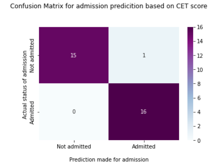
The confusion matrix, an essential tool in evaluating the performance of a classification model, encompasses elements representing True Positive, True Negative, False Positive, and False Negative values. One can generate this matrix by utilizing the code provided below, facilitating a clear understanding of the model’s predictive accuracy and errors. Furthermore, validation techniques ensure the model’s robustness, guard against overfitting, and enhance its generalization capabilities.

#Creating confusion matrix
ConfusionMatrix = confusion_matrix(y_test, y_pred)
print(ConfusionMatrix)

ax = sns.heatmap(ConfusionMatrix, annot=True, cmap='BuPu')
ax.set_title('Confusion Matrix for admission predicition based on CET scorenn');
ax.set_xlabel('nPrediction made for admission')
ax.set_ylabel('Actual status of admission ');
## Ticket labels - List must be in alphabetical order
ax.xaxis.set_ticklabels(['Not admitted','Admitted'])
ax.yaxis.set_ticklabels(['Not admitted','Admitted'])
## Display the visualization of the Confusion Matrix.
plt.show()

Output:

• True Positive: The number of predictions made for admission is “Admitted,” and the actual status of the entry is also “Admitted”. In this case, True Positive= 16.
• True Negative: The number of predictions made for admissions is “Not Admitted,” and the actual status of the entrance is also “Not admitted.”

Similarly, a False Positive is several predictions made for “Admitted” when “ Here, the False the status was Positive is 1. False Negatives can be obtained similarly. Now, accuracy is given by several true predictions divided by the total number of predictions made. From the above confusion matrix, the accuracy rate is =31/32= 0.96875.

Following code can be used to obtain the accuracy rate-

#Accuracy from confusion matrix
TP= ConfusionMatrix[1,1] #True positive
TN= ConfusionMatrix[0,0] #True negative
Total=len(y_test)
print("Accuracy from confusion matrix is ", (TN+TP)/Total)

Step 9: Obtain the regression coefficients using the statsmodel package

#Using statsmodels package to obtian the model
import statsmodels.api as sm
x_train = sm.add_constant(x_train)
logit_model=sm.Logit(y_train,x_train)
result=logit_model.fit()
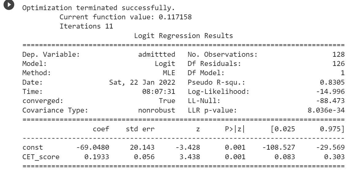
print(result.summary())

Output:

It is seen from the figSize that the same values of the regression coefficients are obtained.

Step 10: Interpreting the value of coefficient b1 in terms of odds ratio

Let us calculate the log of odds for CET_Score= 372 and 373.

ln(Odds(372))= b0+b1*372= -69.048+0.1933*372= 2.8596

ln(Odds(373)= b0+b1*373=-69.048+0.1933*373=3.0529

Now taking difference of both the odds,

ln(Odds(373)) - ln(Odds(372)) = 3.0529-2.8596= 0.1933=b1

Therefore the Odd Ratio is

ln(Odds(373)/Odds(372))= b1

Taking antilog on both the sides:

Odds(373)/Odds(372)= e^b1

Odds(373)/Odds(372)= e^0.1933

Odds(373)/Odds(372)= 1.2132

Therefore, the odds increase by 21.3% for everyone’s mark increase in the CET score.

Let us take one more example: We want to compare candidate A’s 340 marks to candidate B’s 355 marks in terms of odd ratio.

Odds Ratio= Odds(355)/Odds(340)= e^(355-340)b1= e^15b1=  18.165.

So, Candidate B’s odds of getting admission are approximately 18 times higher than Candidate A’s

Conclusion

In this article, we have read about the intricacies of logistic regression, both in theory and practice. Beginning with a fundamental grasp of the mathematical underpinnings, we progressed to practical implementation in Excel and Python. By elucidating the interpretation of regression coefficients through odds ratios, we’ve aimed to provide a comprehensive understanding. Moreover, we’ve also explored the evaluation of our logistic regression model using a classification report, which offers valuable insights into its performance. Additionally, for those eager to dive deeper, we’ve included Python code and a dataset to facilitate hands-on learning and experimentation with logistic regression.

Read more articles on Logistic Regression on our blog.

Frequently Asked Questions

The media shown in this article is not owned by Analytics Vidhya and are used at the Author’s discretion.