Introduction
The main idea of this article is to help you all understand the concept of Sentiment Analysis Deep Learning & NLP. Let’s try to understand this with the help of a case. Anirudh owns an e-commerce company-Universal for the past 1 year and he was very happy as more and more new customers were coming to purchase through his platform. One day he came to know that one of his friends was not satisfied with the product he purchased through his platform. He purchased a foldable geared cycle and the parts required for assembly were missing. He saw few negative reviews by other customers but he purchased from Anirudh as he was his friend. After listening to his friend, Anirudh decided to deploy a machine-learning algorithm to categorize user reviews and their sentiments so that his team can understand their customers better and provide the products and services without any inconvenience to the customers.
Goal: To know what users are saying about products and services. It can help in future decision-making.
Objective: 1. To compile and Tag past data of User Reviews.
2. Use of NLP and Deep Learning to classify the Reviews and find out the Polarity/Sentiment.
His Team labelled the past User Review data. They were reading the Reviews and Classifying them into one or more categories.
1 indicates the presence of that category. For Example, First Review is talking about usability and its polarity/sentiment is negative as the user is complaining(indicated by 0) whereas the second review is talking about features and Functionality having a positive Polarity/Sentiment(indicated by 1)

Anant is the Data Scientist in the company. Now it’s his time to be in the playground. He is using Jupyter Notebook for the model building.
Getting Familiar with Data
Importing Core Libraries
1 import pandas as pd
2 import numpy as np
3 import matplotlib.pyplot as plt                        # For Plotting
4 import seaborn as sns                                  # For Plotting
5 from sklearn.metrics import log_loss                   # For Model Evaluation
6 from sklearn.model_selection import RepeatedKFold      # For Cross-Validation
Reading data
data = pd.read_csv("/content/train.csv")
data.head()                                 # First 5 rows

Observation: By looking at the data, it is clear that it has multiclass(12 classes). It is called a multiclass problem. Apart from multiclass a review can have >=1 category. For Example, Id-1 has 2 categories, Features & Functionality. Categories are not mutually exclusive which is called multilabel. By combining both, we can say that it is a multiclass, multilabel challenge.
data.columns # List of columns in the dataframe

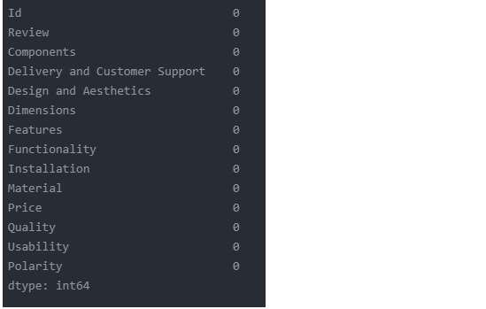
data.isnull().sum()

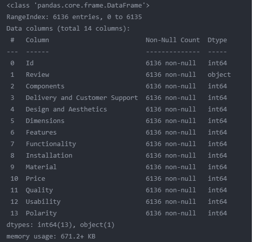
data.info()

data.shape

Exploratory Data Analysis (EDA)
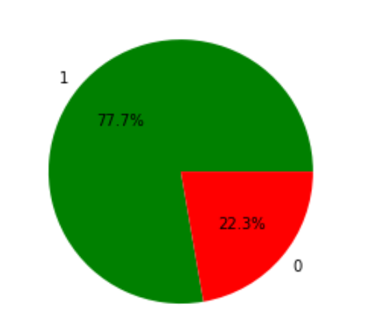
What % of users are talking negatively about the product/services?
sentiment_count = data.Polarity.value_counts()
sentiment_type = data.Polarity.value_counts().index                # 1- Positive    0- Negative
plt.pie(sentiment_count,lablels=sentiment_type, autopct='1.1f%%',colors=['green', 'red'])

Observation: 22.3 % of users are giving negative reviews. In simple terms, only 1 out 5 users are giving negative reviews.
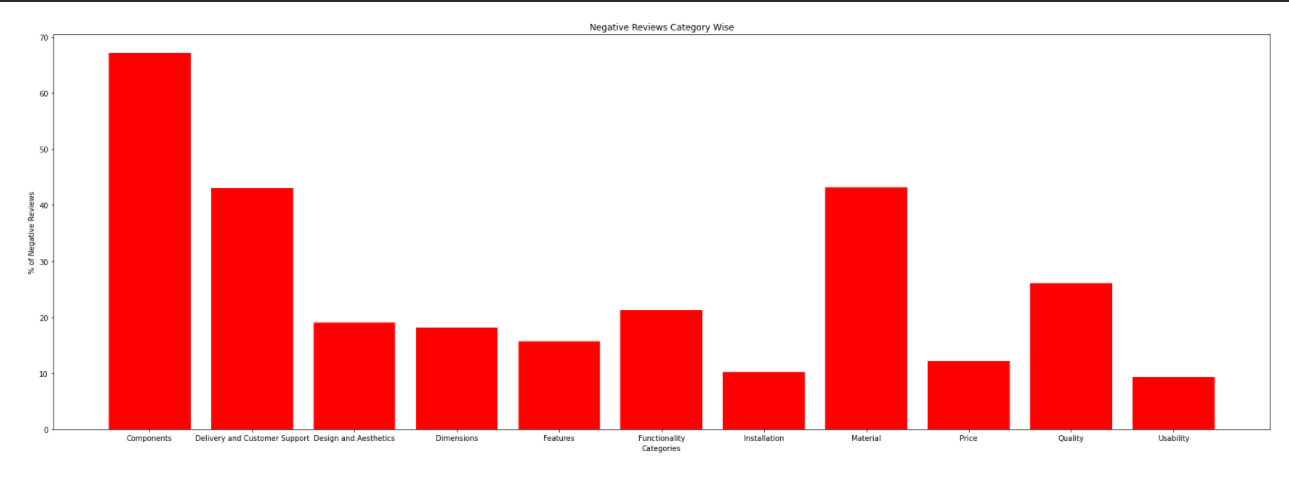
Out of total Reviews in different categories, What % of reviews are negative in different categories?
col = ['Components', 'Delivery and Customer Support',
       'Design and Aesthetics', 'Dimensions', 'Features', 'Functionality',
       'Installation', 'Material', 'Price', 'Quality', 'Usability']
negative_category=[]
for i in col:
    k = ((data[i].sum()-data[data[i]==1]['Polarity'].sum())/data[i].sum())*100
    negative_category.append(k)
fig = plt.figure(figsize = (30, 10))
plt.bar(col,negative_category,color ='red')
plt.xlabel("Categories")
plt.ylabel("% of Negative Reviews")
plt.title("Negative Reviews Category Wise")
plt.show()

Observation: Out of total reviews in different categories, Users are giving the highest % of negative reviews for the Component Category. This is followed by Material, Delivery, and Customer Support.
Text Preprocessing in NLP
Before we feed our data as input to the machine learning algorithm, it’s important to prepare the data in such a way that it reduces the time for processing, takes less memory space, and gives the highest metric evaluation.
Lower Casing & De contraction
The lower casing is removing capitalization from words so that it is treated the same. For example, Look & look are considered different as the first one is capitalized.
import re
def clean_text(text):
    text = text.lower()
    text = re.sub(r"what's", "what is ", text)
    text = re.sub(r"'s", " ", text)
    text = re.sub(r"'ve", " have ", text)
    text = re.sub(r"can't", "can not ", text)
    text = re.sub(r"n't", " not ", text)
    text = re.sub(r"i'm", "i am ", text)
    text = re.sub(r"'re", " are ", text)
    text = re.sub(r"'d", " would ", text)
    text = re.sub(r"'ll", " will ", text)
    text = text.strip(' ')

    return text

Stop Words Removal
Stop words are used for grammatical flow and connecting sentences. For example, I ,are, my, me etc. It does not convey any meaning. If we get rid of stop words, we can reduce the size of our data without information loss. NLTK library is used here to remove stop words.
!pip install nltk
import nltk
from nltk.corpus import stopwords
stop_words = stopwords.words('english')
data['Review'] = data['Review'].apply(lambda x: ' '.join([word for word in x.split() if word not in (stop_words)]))
data['Review'][0]

y = np.array(data[[ 'Components', 'Delivery and Customer Support',
       'Design and Aesthetics', 'Dimensions', 'Features', 'Functionality',
       'Installation', 'Material', 'Price', 'Quality', 'Usability','Polarity']])
X = data['Review']
X.head(5)

X.shapes

Feature Matrix through TF-IDF
from sklearn.feature_extraction.text import TfidfVectorizer
vectorizer = TfidfVectorizer(min_df=20,ngram_range=(1,4), max_features=250)
vectorizer.fit(X)
X = vectorizer.transform(X)  # Taking X as input and converting into feature matrix(numerical values)
X = X.todense()
Deep Learning in Picture
Deep learning attempts to mimic the human brain, and analysis with deep learning fetches fruitful results when we implement it in our model. In deep learning, there are at least three hidden layers. Each unit that takes, processes or outputs the data is called a neuron just like we have in our brain. Based on the work these neurons do, deep learning neurons are divided into input, hidden & output layers. More Hidden layers mean a more complex model!
!pip install tensorflow
from tensorflow.keras.models import Sequential
from tensorflow.keras.layers import Dense, Activation, Dropout
from tensorflow.keras.initializers import RandomNormal
def get_model(n_inputs, n_outputs):
  batch_size = 256
  hidden_units = 64
  dropout = 0.2

  model = Sequential()
  model.add(Dense(hidden_units, input_dim=n_inputs,activation='relu',
          kernel_initializer='he_uniform'))
  model.add(Dropout(dropout))
  model.add(Dense(64,activation='relu',
          kernel_initializer='he_uniform'))
  model.add(Dropout(dropout))
  model.add(Dense(n_outputs))
  model.add(Activation('sigmoid'))
  model.compile(loss='binary_crossentropy', optimizer='adam')
  return model
import tensorflow as tf
def evaluate_model(X,y):
  results_test = []
  results_train =[]
  callback = tf.keras.callbacks.EarlyStopping(monitor='loss', patience=5,min_delta = 0.05)
  n_inputs, n_outputs = X.shape[1], y.shape[1]
  cv = RepeatedKFold(n_splits=10, n_repeats=3, random_state=1)
  for train_ix,test_ix in cv.split(X):
    X_train, X_test = X[train_ix], X[test_ix]
    y_train,y_test = y[train_ix],y[test_ix]
    model = get_model(n_inputs, n_outputs)
    model.fit(X_train,y_train,verbose = 0,epochs = 50,callbacks = callback)
    yhat_train = model.predict(X_train)
    yhat_test = model.predict(X_test)
    train_log_loss = log_loss(y_train, yhat_train)
    test_log_loss = log_loss(y_test,yhat_test)
    results_train.append(train_log_loss)
    results_test.append(test_log_loss)
  return results_train,results_test,model
results_train,results_test,model = evaluate_model(X, y)
print(results_train)
print(results_test)

Training and Validation Score
print(sum(results_train)/len(results_train)
print(sum(results_test)/len(results_test)
Training Log Loss = 3.45
Cross-Validation Log Loss = 3.69
Its time to test on current User Reviews
test_data = pd.read_csv("/content/test.csv")
test_data.head(5)

Preprocessing
test_data['Review'] = test_data['Review'].map(lambda com : clean_text(com))
test_data['Review'] = test_data['Review'].apply(lambda x: ' '.join([word for word in x.split() if word not in (stop_words)]))
test_vectorised_data = vectorizer.transform(test_data['Review'] )
test_vectorised_data = test_vectorised_data.todense()
Prediction on Test Data
prediction_on_test_data = model.predict(test_vectorised_data)
df_test = pd.DataFrame(prediction_on_test_data, columns = ['Components', 'Delivery and Customer Support',
       'Design and Aesthetics', 'Dimensions', 'Features', 'Functionality',
       'Installation', 'Material', 'Price', 'Quality', 'Usability',
       'Polarity'])
df_test

Conclusion
Let’s check a few Reviews classification and Polarity Suggested by our Model
Review: Made of very thin cheap metal broke on the very first crimp. Had to rush to a local hardware store spend 60 more on another because the water was shut off in my home.Did not return because using the case for the new one.
Our Model is categorizing it as Quality- 0.86 and Polarity/Sentiment-0.06(Negative)
Review: As good as the brand names, no jams or misfires on my Paslode fuel cell nailer or on my Banks (HF) nailer.
Our Model is categorizing it as Functionality- 0.79 and Polarity/Sentiment-0.88(Positive)
Different departments now can take actions based on negative reviews in their bucket.
Thus from the above article, it has been lucidly explained as to how we can categorise user reviews and and study the sentiment analysis with Deep Learning & NLP.
The media shown in this article is not owned by Analytics Vidhya and are used at the Author’s discretion.


