Fake News Classification Using Deep Learning

This article was published as a part of the Data Science Blogathon.

Introduction

Here’s a quick puzzle for you. I’ll give you two titles, and you’ll have to tell me which is fake. Ready? Let’s get started:

“Adani Group is planning to explore investment in the EV sector.”
“Wipro is planning to buy an EV-based startup.”

Well, it turns out that both of those headlines were fake news. In this article, you will learn the fake news classification using deep learning.

The grim reality is that there is a lot of misinformation and disinformation on the internet. Ninety per cent of Canadians have fallen for false news, according to a 2019 research done by Ipsos Public Affairs for Canada’s Centre for International Governance Innovation.

It got me thinking: is it feasible to build an algorithm that can tell whether an article’s title is fake news? Well, it appears to be the case!

In this post, we go through the exploration of the classification model with BERT and LSTMs to identify the fake new classification.

Go through this Github link to view the complete code.

Dataset for Fake News Classification

We use the dataset from Kaggle. It consists of 2095 article details that include author, title, and other information. Go through the link to get the dataset.

EDA

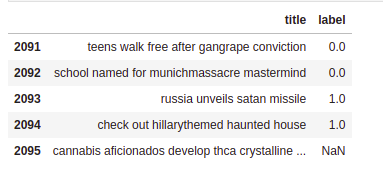
Let us start analyzing our data to get better insights from it. The dataset looks clean, and now we map the values to our class Real and Fake such as 0 and 1.

data = pd.read_csv('/content/news_articles.csv')
data = data[['title', 'label']]
data['label'] = data['label'].map({'Real': 0, 'Fake':1})
data.head()

Since we have 1294 samples of real news and 801 samples of fake news, there is an approximately 62:38 news ratio. It means that our dataset is relatively biased. For our project, we consider the title and class columns.

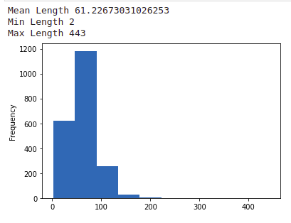
Now, we can analyze the trends present in our dataset. To get an idea of dataset size, we get the mean, min, and max character lengths of titles. We use a histogram to visualize the data.

# Character Length of Titles - Min, Mean, Max
print('Mean Length', data['title'].apply(len).mean())
print('Min Length', data['title'].apply(len).min())
print('Max Length', data['title'].apply(len).max())

x = data['title'].apply(len).plot.hist()

We can observe that characters in each title range from 2-443. We can also see that more per cent of samples with a length of 0-100. The mean length of the dataset is around 61.

Preprocessing Data

Now we will use the NLTK library to preprocess our dataset, which includes:

Tokenization:

It is the process of dividing a text into smaller units (each word will be an index in an array)

Lemmatization:

It removes the endings of the word to the root word. It reduces the word children to a child.

Stop words Removal:

Words like the and for will be eliminated from our dataset because they take too much room.

#Import nltk preprocessing library to convert text into a readable format
import nltk
from nltk.tokenize import sent_tokenize
from nltk.stem import WordNetLemmatizer 
from nltk.corpus import stopwords

nltk.download('punkt')
nltk.download('wordnet')
nltk.download('stopwords')

#Tokenize the string (create a list -> each index is a word)
data['title'] = data.apply(lambda row: nltk.word_tokenize(row['title']), axis=1)

#Define text lemmatization model (eg: walks will be changed to walk)
lemmatizer = WordNetLemmatizer()

#Loop through title dataframe and lemmatize each word
def lemma(data):
  return [lemmatizer.lemmatize(w) for w in data]

#Apply to dataframe
data['title'] = data['title'].apply(lemma)

#Define all stopwords in the English language (it, was, for, etc.)
stop = stopwords.words('english')

#Remove them from our dataframe
data['title'] = data['title'].apply(lambda x: [i for i in x if i not in stop])

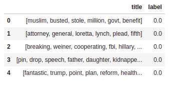
data.head()

We create two models using this data for text classification:

• An LSTM model (Tensorflow’s wiki-words-250 embeddings)
• A BERT model.

LSTM Model for Fake News Classification

We split our data into a 70:30 ratio of train and test.

#Split data into training and testing dataset
title_train, title_test, y_train, y_test = train_test_split(titles, labels, 
                                                            test_size=0.3, 
                                                            random_state=1000)

To get predictions based on the text from our model, we need to encode it in vector format then it is processed by the machine.

Word2Vec Skip-Gram architecture had used by TensorFlow’s wiki-words-250. Based on the input, Skip-gram had trained by predicting the context.

Consider this sentence as an example:

I am going on a voyage in my car.

The word voyage passed as input and one as the window size. The window size means before and after the target word to predict. In our case, the words are gone and car (excluding stopwords, and go is the lemmatized form of going).

We one-hot-encode our word, resulting in an input vector of size 1 x V, where V is the vocabulary size. A weight matrix of V rows (one for each word in our vocabulary) and E columns, where E is a hyperparameter indicating the size of each embedding, will be multiplied by the representation. Except for one, all values in the input vector are zero because it is one-hot encoded (representing the word we are inputting). Finally, when the weight matrix had multiplied by the output, a 1xE vector denotes the embedding for that word.

The output layer, which consists of a softmax regression classifier, will receive the 1xE vector. It had built of V neurons (which correspond to the vocabulary’s one-hot encoding) that produce a value between 0 and 1 for each word, indicating the likelihood of that word being in the window size.

Word embeddings with a size E of 250 are present in Tensorflow’s wiki-words-250. Embeddings applied to the model by looping through all of the words and computing the embedding for each one. We’ll need to utilize the pad sequences function to adjust for samples of variable lengths.

embed = hub.load("https://tfhub.dev/google/Wiki-words-250/2")

#Convert each series of words to a word2vec embedding
indiv = []
for i in title_train:
  temp = np.array(embed(i))
 
  indiv.append(temp)

#Accounts for different length of words
indiv = tf.keras.preprocessing.sequence.pad_sequences(indiv,dtype='float')
indiv.shape

Therefore, there are 1466 samples in the training data, the highest length is 46 words, and each word has 250 features.

Now, we build our model. It consists of:

• 1 LSTM layer with 50 units
• 2 Dense layers (first 20 neurons, the second 5) with an activation function ReLU.
• 1 Dense output layer with activation function sigmoid.

We will use the Adam optimizer, a binary cross-entropy loss, and a performance metric of accuracy. The model will be trained over 10 epochs. Feel free to further adjust these hyperparameters.

#Sequential model has a 50 cell LSTM layer before Dense layers
model = tf.keras.models.Sequential()


model.add(tf.keras.layers.LSTM(50))
model.add(tf.keras.layers.Dense(20,activation='relu'))
model.add(tf.keras.layers.Dense(5,activation='relu'))

model.add(tf.keras.layers.Dense(1,activation='sigmoid'))

#Compile model with binary_crossentropy loss, Adam optimizer, and accuracy metrics
model.compile(optimizer=tf.keras.optimizers.Adam(learning_rate = 1e-4),
              loss="binary_crossentropy", metrics=['accuracy'])

#Train model on 10 epochs
model.fit(indiv, y_train,validation_data=[test,y_test], epochs=20)

We get an accuracy of 59.4% on test data.

Using BERT for Fake News Classification

What would you reply if I asked you to name the English term with the most definitions?

That word is “set,” according to the Oxford English Dictionary’s Second Edition.

If you think about it, we could make a lot of different statements using that term in various settings. Consider the following scenario:

My books are part of a set of stationery collections
My teammate set the badminton for me
I set the table for lunch

The problem with Word2Vec is that no matter how the word had used, it generates the same embedding. We use BERT, which can build contextualized embeddings, to combat this.

BERT is known as “Bidirectional Encoder Representations from Transformers.” It employs a transformer model to generate contextualized embeddings by utilizing attention mechanisms.

An encoder-decoder design had used in a transformer model. The encoder layer creates a continuous representation based on the data it has learned from the input. The preceding input is delivered into the model by the decoder layer, which generates an output. Because BERT’s purpose is to build a vector representation from the text, it only employs an encoder.

Pre-Training & Fine-Tuning

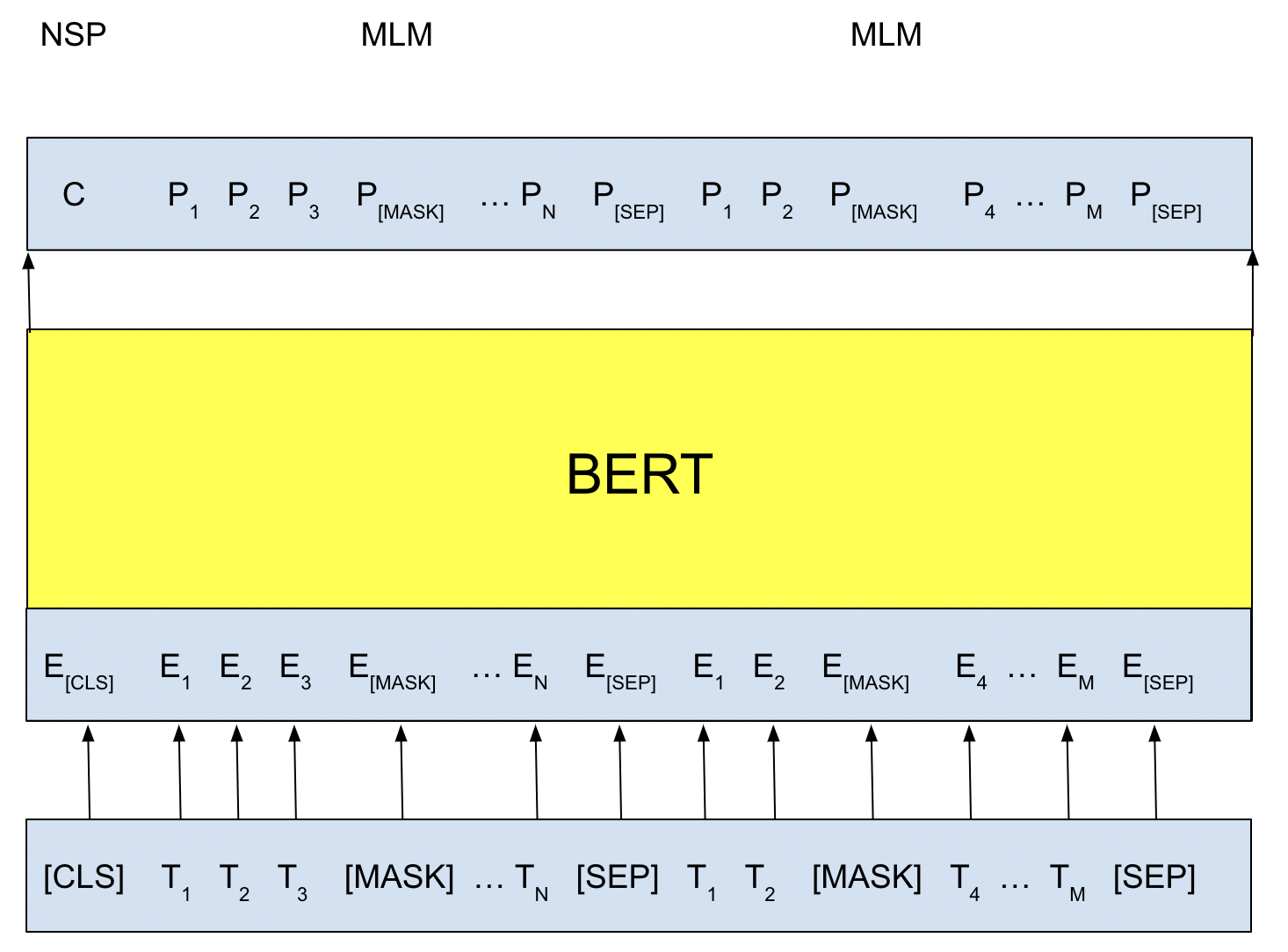
BERT had trained using two ways. The first method is known to be veiled language modelling. Before transmitting sequences, a [MASK] token had used to replace 15% of the words. Using the context supplied by the unmasked words, the model will predict the masked words.

• Using embedding matrix to apply a classification layer to the encoder output. As a result, it will be the same size as the vocabulary.
• Using the softmax function to calculate the likelihood of the word.

The second strategy is to guess the upcoming sentence. The model will be given two sentences as input and predict whether the second sentence will come after the first. While training, half of the inputs are pairs, while the other half consists of random sentences from the corpus. To distinguish between the two statements,

• Here, it adds a [CLS] token at the start of the first sentence and a [SEP] token at the end of each.
• Each token (word) contains a positional embedding that allows information extracted from the text’s location. Because there is no repetition in a transformer model, there is no inherent comprehension of the word’s place.
• Each token is given a sentence embedding (further differentiating between the sentences).

For Next Sentence Prediction, the output of the [CLS] embedding, which stands for “aggregate sequence representation for sentence classification,” is passed through a classification layer with softmax to return the probability of the two sentences being sequential.

Image by Author

Implementation of BERT

The BERT preprocessor and encoder from Tensorflow-hub had used. Do not run the content via the earlier-mentioned framework (which removes capitalization, applies lemmatization, etc.) The BERT preprocessor had used to abstract this.

We split our data for training and testing in the ratio of 80:20.

from sklearn.model_selection import train_test_split  
#Split data into training and testing dataset 
title_train, title_test, y_train, y_test = train_test_split(titles, labels, test_size=0.2,                                                             random_state=1000)

Now, load Bert preprocessor and encoder

# Use the bert preprocesser and bert encoder from tensorflow_hub 
bert_preprocess = hub.KerasLayer("https://tfhub.dev/tensorflow/bert_en_uncased_preprocess/3") 
bert_encoder = hub.KerasLayer('https://tfhub.dev/tensorflow/bert_en_uncased_L-12_H-768_A-12/4')

We can now work on our neural network. It must be a functional model, with each layer’s output serving as an argument to the next.

• 1 Input layer: Used to pass sentences into the model.
• The bert_preprocess layer: Preprocess the input text.
• The bert_encoder layer: Pass the preprocessed tokens into the BERT encoder.
• 1 Dropout layer with 0.2. The BERT encoder pooled_output is passed into it.
• 2 Dense layers with 10 and 1 neurons. The first uses a ReLU activation function, and the second is sigmoid.

import tensorflow as tf

# Input Layers
input_layer = tf.keras.layers.Input(shape=(), dtype=tf.string, name='news')

# BERT layers
processed = bert_preprocess(input_layer)
output = bert_encoder(processed)

# Fully Connected Layers
layer = tf.keras.layers.Dropout(0.2, name='dropout')(output['pooled_output'])
layer = tf.keras.layers.Dense(10,activation='relu', name='hidden')(layer)
layer = tf.keras.layers.Dense(1,activation='sigmoid', name='output')(layer)


model = tf.keras.Model(inputs=[input_layer],outputs=[layer])

The “pooled output” will be transmitted into the dropout layer, as you can see. This value represents the text’s overall sequence representation. It is, as previously said, the representation of the [CLS] token outputs.

The Adam optimizer, a binary cross-entropy loss, and an accuracy performance metric had used. For five epochs, the model had trained. Feel free to tweak these hyperparameters even more.

#Compile model on adam optimizer, binary_crossentropy loss, and accuracy metrics
model.compile(optimizer='adam',loss='binary_crossentropy',metrics=['accuracy'])
#Train model on 5 epochs
model.fit(title_train, y_train, epochs= 5)

#Evaluate model on test data
model.evaluate(title_test,y_test)

Image by Author

Above, you can see that our model achieved an accuracy of 61.33%.

Conclusion

To improve the model performance:

• Train the models on a large dataset.
• Tweak hyperparameters of the model.

I hope you had found this post insightful and a better understanding of NLP techniques for fake news classification.

Read more articles on our blog. Click here.

References

Image – 1: Photo by Roman Kraft on Unsplash

The media shown in this article is not owned by Analytics Vidhya and are used at the Author’s discretion. 

Pavan Kalyan 22 Mar 2022

Myself Pavan Kalyan with 2 years of experience in developing, deploying scalable Machine Learning models and interested to explore data, discover useful insights. I like to participate in the Machine Hack and Kaggle competitions.