Understand the Realtime Image Classification: CNN

This article was published as a part of the Data Science Blogathon.

An end-to-end guide on classifying facial emotion in real-time using deep learning.

Hey readers!

In the last article, we had talked about the facial attendance system. In this article, we will talk about how can we integrate emotion detection in our project in real-time scanning.

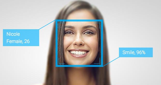
Facial emotion recognition is a computer vision (CV) job, and it can be done on a bunch of images or can be done in real-time.

As we all see (CV) is getting more robust, companies are adopting its leading technological features to get their job done faster and with accuracy.

This article explains how to build a TensorFlow model to categorize facial emotions in real-time using a webcam.

Table of Contents

• Downloading data
• Data Preprocessing
• Data Augmentation
• Model building and training
• Integration with OpenCV-Realtime

Introduction

Image detection in real-time is one step further than image detection, integrating image detection with open-cv can let us classify pictures in real-time.

In this article, we will use open-cv and a trained model for classifying the facial emotion in realtime using web-cam

Downloading Data

For the implementation, we are going to use a public dataset on Kaggle that is fer-2013 and it has 48*48 gray-scale pictures of faces with their emotion labels. The dataset contains the values of pixels that we need to process in upcoming steps.

7 Emotions in the Dataset :- (0=Angry, 1=Disgust, 2=Fear, 3=Happy, 4=Sad, 5=Surprise, 6=Neutral)

a. Dataset Loading

Importing necessary libraries including pandas.

##import pandas and numpy
df = pdy.read_csv('../input/facial-expression-recognitionferchallenge/fer2013/fer2013/fer2013.csv')
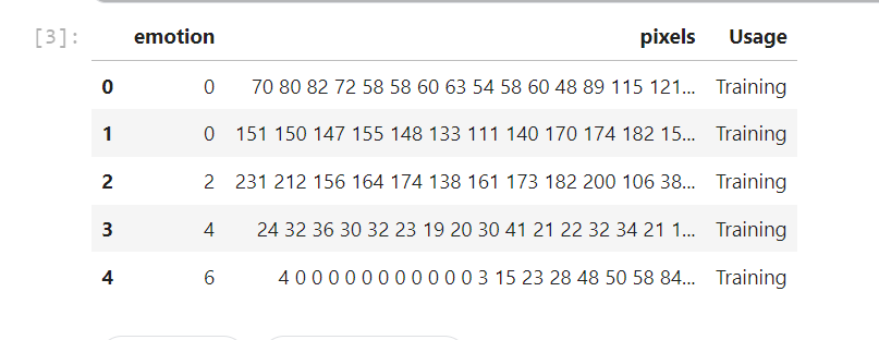
df.head()

 

The dataset includes 3 columns, emotion, pixels, and usage. emotion column is the number of emotion classes, pixels are 48*48 pixels one tab apart in the form of string.

b. Data preprocessing

The dataset is not in the right format, we need to convert the pixels into a numerical array and have to segregate them for the training and testing part.

X_train, X_test will contain the pixels for training and testing images, and y_test,y_train will contain the emotion labels.

X_train = []
y_train = []
X_test = []
y_test = []
for index, row in df.iterrows():
    k = row['pixels'].split(" ")
    if row['Usage'] == 'Training':
        X_train.append(np.array(k))
        y_train.append(row['emotion'])
    elif row['Usage'] == 'PublicTest':
        X_test.append(np.array(k))
        y_test.append(row['emotion'])

As of nowX_train is an array and contains the string, we need to convert it into the integer by type-casting.

X_train = np.array(X_train, dtype = 'uint8')
y_train = np.array(y_train, dtype = 'uint8')
X_test = np.array(X_test, dtype = 'uint8')
y_test = np.array(y_test, dtype = 'uint8')

• y_test,y_train is now an array of integer encoded labels, for better training we need to convert them into a categorical data matrix.

import keras
from keras.utils import to_categorical
y_train= to_categorical(y_train, num_classes=7)
y_test = to_categorical(y_test, num_classes=7)

num_classes = 7 it shows that we have 7 emotion classes.

c. Shaping our data

For performing the training we need a 4d tensor in the form of ( row_num, width, height, channel).

X_train = X_train.reshape(X_train.shape[0], 48, 48, 1)
X_test = X_test.reshape(X_test.shape[0], 48, 48, 1)

• Here 1 indicates that the training data is in grayscale form.
• Now we have our X_train, X_test, y_train,y_test for training and testing.

Data Augmentation

Data Augmentation means creating augmented data ( Synthetic ) using some transformation in order to achieve more generalized training.

Keras provides ImageDataGenerator class that handles all the preprocessing for image augmentation.

from keras.preprocessing.image import ImageDataGenerator 
datagen = ImageDataGenerator( 
    rescale=1./255,
    rotation_range = 10,
    width_shift_range=0.1,
    horizontal_flip = True,
    height_shift_range=0.1,
    fill_mode = 'nearest')

testgen = ImageDataGenerator( 
    rescale=1./255
    )
datagen.fit(X_train)

batch_size = 64

• rescale : normalizes the pixels by diving by a fixed number.
• horizontal_flip : flips the image in the horizontal direction.
• fill_mode : fills the image if after cropping it comes out blank.

Note: For testing, we only need to apply image rescaling.

Training Data Generator

Fitting Data Generator generates the images into a fixed batch size of 64 which can be changed by users.

Data generator solves the problem of insufficient memory for training the big size of data.

train_flow = datagen.flow(X_train, y_train, batch_size=batch_size) 
test_flow = testgen.flow(X_test, y_test, batch_size=batch_size)

• train_flow is X_train and y_train
• test_flow is X_test and y_test

CNN Model Building

We will be using functional API for model building since functional API gives easier layer integration and easier to build models on it.

We will create model blocks using Batch-Normalization, Conv2D layer, Max-Pooling2D, Dropout, Flatten layer and then stack them together at the end using dense layer for output.

For a more detailed description of the model, building read here.

Importing necessary libraries for the model

from keras.utils import plot_model
from keras.models import Model
from keras.layers import Input,Flatten,Dropout,Dense, BatchNormalization
from keras.layers.convolutional import Conv2D
from keras.layers.pooling import MaxPooling2D
from keras.layers.merge import concatenate
from keras.optimizers import Adam, SGD
from keras.regularizers import l1, l2
from sklearn.metrics import confusion_matrix

Model Designing

Creating a function that takes some parameters and returns a model ready for training.

def FER_Model(input_shape=(48,48,1)):
    # first input model
    visible = Input(shape=input_shape, name='input')
    num_classes = 7
    #the a block
    conva_1 = Conv2D(64, kernel_size=3, activation='relu', padding='same', name = 'conva_1')(visible)
    conva_1 = BatchNormalization()(conva_1)
    conva_2 = Conv2D(64, kernel_size=3, activation='relu', padding='same', name = 'conva_2')(conva_1)
    conva_2 = BatchNormalization()(conva_2)
    poola_1 = MaxPooling2D(pool_size=(2,2), name = 'poola_1')(conva_2)
    dropa_1 = Dropout(0.3, name = 'dropa_1')(poola_1)

#the b block
    convb_1 = Conv2D(128, kernel_size=3, activation='relu', padding='same', name = 'convb_1')(dropa_1)
    convb_1 = BatchNormalization()(convb_1)
    convb_2 = Conv2D(128, kernel_size=3, activation='relu', padding='same', name = 'convb_2')(convb_1)
    convb_2 = BatchNormalization()(convb_2)
    convb_3 = Conv2D(128, kernel_size=3, activation='relu', padding='same', name = 'convb_3')(convb_2)
    convb_2 = BatchNormalization()(convb_3)
    poolb_1 = MaxPooling2D(pool_size=(2,2), name = 'poolb_1')(convb_3)
    dropb_1 = Dropout(0.3, name = 'dropb_1')(poolb_1)

#the c block
    convc_1 = Conv2D(256, kernel_size=3, activation='relu', padding='same', name = 'convc_1')(dropb_1)
    convc_1 = BatchNormalization()(convc_1)
    convc_2 = Conv2D(256, kernel_size=3, activation='relu', padding='same', name = 'convc_2')(convc_1)
    convc_2 = BatchNormalization()(convc_2)
    convc_3 = Conv2D(256, kernel_size=3, activation='relu', padding='same', name = 'convc_3')(convc_2)
    convc_3 = BatchNormalization()(convc_3)
    convc_4 = Conv2D(256, kernel_size=3, activation='relu', padding='same', name = 'convc_4')(convc_3)
    convc_4 = BatchNormalization()(convc_4)
    poolc_1 = MaxPooling2D(pool_size=(2,2), name = 'poolc_1')(convc_4)
    dropc_1 = Dropout(0.3, name = 'dropc_1')(poolc_1)

#the d block
    convd_1 = Conv2D(256, kernel_size=3, activation='relu', padding='same', name = 'convd_1')(dropc_1)
    convd_1 = BatchNormalization()(convd_1)
    convd_2 = Conv2D(256, kernel_size=3, activation='relu', padding='same', name = 'convd_2')(convd_1)
    convd_2 = BatchNormalization()(convd_2)
    convd_3 = Conv2D(256, kernel_size=3, activation='relu', padding='same', name = 'convd_3')(convd_2)
    convd_3 = BatchNormalization()(convd_3)
    convd_4 = Conv2D(256, kernel_size=3, activation='relu', padding='same', name = 'convd_4')(convd_3)    convd_4 = BatchNormalization()(convd_4)
    poold_1 = MaxPooling2D(pool_size=(2,2), name = 'poold_1')(convd_4)
    dropd_1 = Dropout(0.3, name = 'dropd_1')(poold_1)
    
    #the e block
    conve_1 = Conv2D(512, kernel_size=3, activation='relu', padding='same', name = 'conve_1')(dropd_1)
    conve_1 = BatchNormalization()(conve_1)
    conve_2 = Conv2D(512, kernel_size=3, activation='relu', padding='same', name = 'conve_2')(conve_1)
    conve_2 = BatchNormalization()(conve_2)
    conve_3 = Conv2D(512, kernel_size=3, activation='relu', padding='same', name = 'conve_3')(conve_2)
    conve_3 = BatchNormalization()(conve_3)
    conve_4 = Conv2D(512, kernel_size=3, activation='relu', padding='same', name = 'conve_4')(conve_3)
    conve_3 = BatchNormalization()(conve_3)
    poole_1 = MaxPooling2D(pool_size=(2,2), name = 'poole_1')(conve_4)
    drope_1 = Dropout(0.3, name = 'drope_1')(poole_1)

#Flatten and output
    flatten = Flatten(name = 'flatten')(drope_1)
    ouput = Dense(num_classes, activation='softmax', name = 'output')(flatten)

# create model 
    model = Model(inputs =visible, outputs = ouput)
    # summary layers
    print(model.summary())
    
    return model

FER_model takes input size and returns a built model for training.

Compiling Model

Defining training parameters:

We will use Adam optimizer with lr= 0.001.

model = FER_Model()
opt = Adam(lr=0.0001, decay=1e-6)
model.compile(loss='categorical_crossentropy', optimizer=opt, metrics=['accuracy'])

If the model’s accuracy doesn’t improve it will decay.

Model Training

Now we are ready with Training, Testing data, and model.

num_epochs = 100  
history = model.fit_generator(train_flow, 
                    steps_per_epoch=len(X_train) / batch_size, 
                    epochs=num_epochs,  
                    verbose=1,  
                    validation_data=test_flow,  
                    validation_steps=len(X_test) / batch_size)

• validation_steps=Total_validation_Samples / Validation_BatchSize
• steps_per_epoch=Total_Training_Samples / Training_BatchSize

The training process will take up time depending on your computer speed.

Saving the Model

We are saving the model in a JSON file and trained weights into .h5

model_json = model.to_json()
with open("model_arch.json", "w") as json_file:
    json_file.write(model_json)
model.save_weights("model_weights.h5")

We need to save the JSON and weights into our desired directory.

Opencv Integration for Real-time Prediction

Testing our model for face detection and their emotions.

a. Loading the Saved model

from tensorflow.keras.models import model_from_json
model = model_from_json(open("model_arch.json", "r").read())
model.load_weights('model_weights.h5')

b. Face detection using haar-cascade

Getting the face position of humans becomes easier using a haarcascade trained file.

you can downloadhaarcascade_frontalface_default using the link.

import cv2
face_haar_cascade = cv2.CascadeClassifier('haarcascade_frontalface_default.xml')

c. Opencv Video capture and processing

Using OpenCV we can take a video feed and perform some preprocessing for our prediction.

capture=cv2.VideoCapture(0)

while capture.isOpened():
    bool_result,frame_feed=capture.read()

height, width , channel = frame_feed.shape

gray_image= cv2.cvtColor(frame_feed, cv2.COLOR_BGR2GRAY)
    faces_detected = face_haar_cascade.detectMultiScale(gray_image )
    try:
        for (x,y, w, h) in faces_detected:
            roi_gray = gray_image[y-5:y+h+5,x-5:x+w+5]
            roi_gray=cv2.resize(roi_gray,(48,48))
            image_pixels = img_to_array(roi_gray)
            image_pixels = np.expand_dims(image_pixels, axis = 0)
            image_pixels /= 255
            predictions = model.predict(image_pixels)
            max_index = np.argmax(predictions[0])
            emotion_detection_dict = ('anger', 'disgust', 'fear', 'happy', 'sad', 'surprise', 'neutral')
            emotion_prediction = emotion_detection_dict[max_index]

• Normalize test images by dividing by 255.
• haar_cascade only accepts grayscale images.
• emotion_prediction is the class label of emotion.

As of now, we have made our function for the detection of emotions, to improve the output we can add some overlay on it.

cap=cv2.VideoCapture(1)

while cap.isOpened():
    bool_result,frame_feed=cap.read()

height, width , channel = frame_feed.shape

#---------------------------------------------------------------------------
    # Creating an Overlay window to write prediction and cofidence

sub_img = frame_feed[0:int(height/6),0:int(width)]

black_rect = np.ones(sub_img.shape, dtype=np.uint8)*0
    res = cv2.addWeighted(sub_img, 0.77, black_rect,0.23, 0)
    FONT = cv2.FONT_HERSHEY_SIMPLEX
    FONT_SCALE = 0.8
    FONT_THICKNESS = 2
    lable_color = (10, 10, 255)
    lable = "Realtime Emotion Detection"
    lable_dimension = cv2.getTextSize(lable,FONT ,FONT_SCALE,FONT_THICKNESS)[0]
    textX = int((res.shape[1] - lable_dimension[0]) / 2)
    textY = int((res.shape[0] + lable_dimension[1]) / 2

# prediction part --------------------------------------------------------------------------
    faces = face_haar_cascade.detectMultiScale(gray_image )
    try:
        for (x,y, w, h) in faces:
            roi_gray = gray_image[y-5:y+h+5,x-5:x+w+5]
            roi_gray=cv2.resize(roi_gray,(48,48))
            image_pixels = img_to_array(roi_gray)
            image_pixels = np.expand_dims(image_pixels, axis = 0)
            image_pixels /= 255
            predictions = model.predict(image_pixels)
            max_index = np.argmax(predictions[0])
            emotion_detection_dict = ('anger', 'disgust', 'fear', 'happy', 'sad', 'surprise', 'neutral')
            emotion_prediction = emotion_detection_dict[max_index]
            cv2.putText(res, "Sentiment: {}".format(emotion_prediction), (0,textY+22+5), FONT,0.7, lable_color,2)
            lable_violation = 'Confidence: {}'.format(str(np.round(np.max(predictions[0])*100,1))+ "%")
            violation_text_dimension = cv2.getTextSize(lable_violation,FONT,FONT_SCALE,FONT_THICKNESS )[0]
            violation_x_axis = int(res.shape[1]- violation_text_dimension[0])
            cv2.putText(res, lable_violation, (violation_x_axis,textY+22+5), FONT,0.7, lable_color,2)
    except :
        pass
    frame[0:int(height/6),0:int(width)] = res
    cv2.imshow('frame', frame)

if cv2.waitKey(1) & 0xFF == ord('q'):
        break

cap.release()
cv2.destroyAllWindows

Conclusion

In this article, we have learned how to perform real-time emotion detection including preprocessing of data, image data augmentation, and use OpenCV for live camera feeds. we used haar cascade for human face detection.

This project can be improved further by some tweaking.

• Using a deeper CNN model can give us better results.
• perform some model tweaking.
• Using stacked pre-trained models.

Get source codes from here.

Read our latest articles on the website.

The media shown in this article is not owned by Analytics Vidhya and are used at the Author’s discretion. 

Abhishek Jaiswal

A data enthusiast exploring the leading technologies related to the data