Recurrent Neural Networks: Digging a bit deeper

This article was published as a part of the Data Science Blogathon.

Introduction

In the former article, we looked at how RNNs are different from standard NN and what was the reason behind using this algorithm. In this article we will dig a bit deeper into RNN, we will see the mathematical details and try to understand it in the most simpler way. We will also look at some of the problems faced by Recurrent Neural Networks. 

As we already know that RNNs are a type of NN that can be used to model sequence data. Theoretically, RNNs, which are made of feedforward networks, are similar to human brains in their behavior. Simply put, recurrent neural networks can prepare for sequential data in a way that other algorithms can’t. Without wasting our time let’s see what goes under the hood behind this algorithm.

Recurrent Neural Networks model in detail

We already saw that in RNN we pass one word at a time, but the machine doesn’t understand words they understand numbers so we can not pass the word directly to our model. So, we need to convert the word into a number. Let’s take our old example “Chirag worked at Microsoft in India”. The first thing to do is to make a vocabulary of words, now this vocabulary will have all the words known to us but we can limit it to a few thousand English words. Let’s say the word “Chirag” appears somewhere at a position “3456” in the vocabulary and the second word appears at some “6969” position.

Now once we have a number for our word, we can feed it to our model but, before we also need to convert this number into One hot representation. One hot representation is a vector where all the values are 0 except at the place “3456” which will be 1, similarly, the one-hot vector representation of 2^nd word will give as follows:

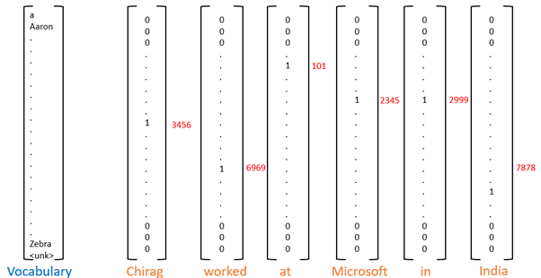
Once we have converted our words into one-hot representation, we can feed them to our network. Now it’s time to understand the nitty-gritty details of this algorithm. In the next section, we will understand what this model does under the hood.

Deep dive into Recurrent Neural Networks

In an ANN, the activation for the next layer was calculated by multiplying the weight to the activation of the past layer and adding some bias to it and then passing it to an activation function.

Let’s do a similar thing for Recurrent Neural networks as well. The equation will be similar only but here we have to inputs, one input is the activation from the previous layer and another input is the word “X” which is some word. In ANN we had only one input so we multiplied only 1 weight matrix but here we have 2 inputs so we will have 2 weight matrices. The equation will look like this:

So the activation from the past timestamp will be multiplied by the weight W_aa and input X which is the word in the numerical form will be multiplied by the weight matrix W_ax. Hence our RNN will look something like this:

Where the equation of Y is

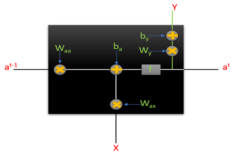
This is our 1 RNN cell and at every time step, we will passwords that will compute some value for the activations and it will produce some output as well. So on a bigger picture, it looks something like this:

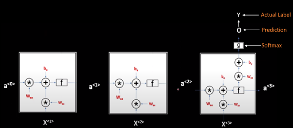
We also saw that for many applications like many-to-one applications we do not have output at every timestamp, but we have output only at the final word. The architecture will look something like this:

Backpropagation in Recurrent Neural Networks

Let’s say we are making a movie rating system in which the purpose is to rate a movie from 1-5 based on the given comment. This problem comes under many to one architecture. To understand backpropagation in RNN, this would be the best architecture to start upon.

The loss function which we will use here is “Categorical Cross Entropy”:

Now let’s understand how backpropagation works in an easier way. We already that in RNN same weight matrix is shared by all the cells at each time step which means W_aa and W_ax is shared through all the timestamps for each cell.

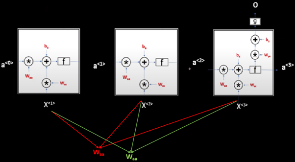
These weight matrices will only be updated at the end of the final timestamp. This means we will move forward through time and when we reach the end of the sentence, we will calculate loss through our loss function, and based on this loss value or error we have our model will try to minimize this error by propagating backward and updating these weights (W_aa, W_ax, and W_ay). WE already know that:

Let’s start by calculating the derivative of loss with respect to W_ya . If you notice closely you’ll notice that Loss is dependent on O, O is dependent on W_ya , chain rule we get:

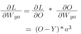
If you don’t understand how this formula came then no need to worry you can just memorize it or try to derive it yourself for practice.

After having the derivative of loss with respect to W_ya you just need to put the value in the weight updating formula which is:

This was the easier part since W_ya shows up only at the final timestamp. A bit more challenging part would be to obtain W_aa and W_ax .

Let’s calculate the derivative of loss w.r.t to W_aa . Here Loss depends on O, O depends on a³ and a³ depends on W_aa . But the story does not end here because if you see that the same W_aa contributes in all the timestamps that mean for obtaining a³ which is the final activation, the activation a^1, and a² have also contributed which again depends on W_aa .

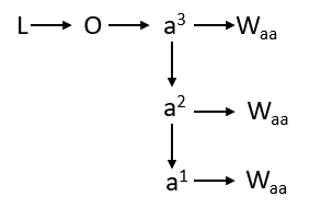
We need to draw our attention to this chain, now let’s backpropagate or use the chain rule in this structure.

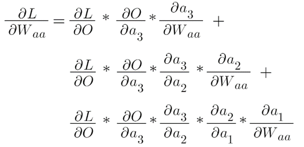
This whole equation can be written as:

Similarly, we can calculate the derivative of loss w.r.t W_ax since they both share the same story.

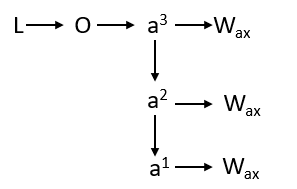
Hence the equation will be:

Thus, we have acquired all the 3 equations necessary for the backpropagation in RNN.

Problems in Recurrent Neural Networks

Let’s say we are making a grammar checker which checks if the given sentence is grammatically correct or not. For example, you input your sentence in your app and this comes to the output, “I just want you to know that if you are out there and you are being really hard on herself right now for something that has happened … it’s normal”

Now clearly here instead of “herself” it should have been “yourself”. This means if we use RNN for creating a Grammar checker then this NN should suggest that here it should be “yourself” not “herself” but practically RNNs are not able to do so. Let’s see why?

Suppose we pass the sentence to this RNN, all the words will go one by one as an input to this RNN but when we pass this long sentence to the RNN it will fail to identify this as an error.

What happens in RNN is that these hidden states which are being passed on to the next timestamp are updated on every timestamp. So by the time, it reaches the end of the sentence or where the error is, the value of the a is updated so many times that it has almost lost the information that was present when it saw the first word or the context of the sentence. That is why the problem with the RNN is that whenever we pass a long sentence it loses the information that was present very earlier in the sentence. It remembers the information from the last few words, but it fails to remember the words or information that showed up long before.

This can also be understood with the help of backpropagation. We derived the derivative of loss w.r.t weight, which came out to be:

If we expand this, we get this as an equation:

This means when we are backpropagating from the time stamp T=t to the time stamp T=1, we have to multiply a lot of gradients to reach the time stamp T=1 and we are also aware that in what range the value of the gradients lies, it is from 0-1, which means that the gradient value is a small number and if a small number is multiplied again and again it becomes almost close to 0, which means while updating the weights which is actual training of our model the words that appear at the earlier stage has almost no say and this problem is known as “Vanishing gradient problem”.

End Notes

In this article, we had an understanding of what RNNs are doing under the hood. We looked at how backpropagation works in this algorithm. We then looked at the problems faced by RNNs and why we don’t use it anymore. In the next article will see and understand how LSTM’s and GRU’s tackle these problems. Before I end this article here are a few implementation details about building an RNN.

• For the first RNN block, since we have no previous hidden state available, it is common to input a vector of zeros.
• While inputting texts of varying lengths we pad each text to make each sequence of equal lengths.
• To specify the start and end of a sentence we can and tokens.

I hope after reading this some doubts regarding RNN might have cleared. Do reach out in the comments if you still have any doubts.

About the Author

Anshul

I have recently graduated with a Bachelor's degree in Statistics and am passionate about pursuing a career in the field of data science, machine learning, and artificial intelligence. Throughout my academic journey, I thoroughly enjoyed exploring data to uncover valuable insights and trends.

I am eager to continue learning and expanding my knowledge in the field of data science. I am particularly interested in exploring deep learning and natural language processing, and I am constantly seeking out new challenges to improve my skills. My ultimate goal is to use my expertise to help businesses and organizations make data-driven decisions and drive growth and success.