5 Python Libraries for Time-Series Analysis

Introduction on Time-Series

A Time-Series is a sequence of data points collected at different timestamps. These are essentially successive measurements collected from the same data source at the same time interval. Further, we can use these chronologically gathered readings to monitor trends and changes over time. The time-series models can be univariate or multivariate. The univariate time series models are implemented when the dependent variable is a single time series, like room temperature measurement from a single sensor. On the other hand, a multivariate time series model can be used when there are multiple dependent variables, i.e., the output depends on more than one series. An example for the multivariate time-series model could be modelling the GDP, inflation, and unemployment together as these variables are linked to each other.

Therefore, the time-series data is valuable as its analysis allows us to analyze past events and help us make predictions for the future (also known as forecasting). The models built using this kind of data are known as Time-series models. The insights from such historical data analysis can uncover trends and patterns helpful in predicting likely future events in business. Most businesses experience seasonality in sales and gaining deeper insights using visualization into these trends enables them to make better business decisions. Predictive analytics and time-series forecasting are essential for businesses to stay ahead of the competition with better planning.

Data for Time Series Analysis

Time-series analysis is generally performed on non-stationary data, i.e., data changing over time. We can find such variable data in the finance domain as currency and stock prices change dynamically. Similarly, weather data like temperature, rainfall, and wind speeds are constantly changing in meteorology. In the healthcare field, monitoring vital parameters of the brain and heart for patients assists in refining the treatment. These are just a few examples, and time-series analysis has broad applicability in several domains.

With the advancements in AI, especially Machine learning, big data processing is possible. So, analyzing time series has become more accessible. Various open-source tools can quickly uncover patterns and deviations from the normal readings. There are multiple time-series analysis techniques like AR (AutoRegressive), MA (Moving Average), ARIMA (Auto-Regressive Integrated Moving Average), Seasonal AutoRegressive Integrated Moving Average (SARIMA), etc. In this article, we will briefly explore five open-source python libraries developed for time series analysis with sample data for forecasting.

Time series analysis with Python Libraries

This article only focuses on the libraries and their python code. Hence, to explore these libraries, it is expected to have at least some theoretical knowledge about time series, the analysis methods or techniques to understand the results, and how to use them. Nevertheless, all these libraries require a few lines of code for the analysis, so they are easy to implement for a beginner. We begin with importing the essential packages for this tutorial.

import matplotlib.pyplot as plt
import pandas as pd
import numpy as np
import seaborn as sns
import plotly

Now, let us look at the libraries in the following section.

1) Tsfresh

The name of this library, Tsfresh, is based on the acronym “Time Series Feature Extraction Based on Scalable Hypothesis Tests.” It is a Python package that automatically calculates and extracts several time series features (additional information can be found here) for classification and regression tasks. Hence, this library is mainly used for feature engineering in time series problems and other packages like sklearn to analyze the time series.

We’ll install this library using –

pip install tsfresh

Since we previously imported the necessary packages, we will now import tsfresh and its functions required for this tutorial.

from tsfresh import extract_features, extract_relevant_features, select_features
from tsfresh.utilities.dataframe_functions import impute, make_forecasting_frame
from tsfresh.feature_extraction import ComprehensiveFCParameters, settings

We will use a standard dataset of Air passengers within 11 years (1949- 1960). This dataset comprises monthly totals of US airline passengers. We can read the dataset into a dataframe using the following lines of code.

# Reading the data
data = pd.read_csv('../input/airline-passengers.csv')

This dataset contains 144 samples with 2 attributes, i.e., Month and Passengers. Let us print a few rows of this dataset using data.head() command

Next, we will use the ‘make_forecasting_frame’ function to extract the features from this time series data.

data.columns = ['month','#Passengers']
data['month'] = pd.to_datetime(data['month'],infer_datetime_format=True,format='%y%m')
df_pass, y_air = make_forecasting_frame(data["#Passengers"], kind="#Passengers", max_timeshift=12, rolling_direction=1)
print(df_pass)

import pandas as pd

from tsfresh.utilities.dataframe_functions import make_forecasting_frame

data = pd.read_csv('AirPassengers.csv')

data.columns = ['month','#Passengers']
data['month'] = pd.to_datetime(data['month'],infer_datetime_format=True,format='%y%m')
df_pass, y_air = make_forecasting_frame(data["#Passengers"], kind="#Passengers", max_timeshift=12, rolling_direction=1)
print(df_pass)

The tsfresh package extracted 143 rows with 789 features. This shows how quickly tsfresh identified features from the sequential input data. It is possible to further narrow this extracted feature dataset by removing any non-values in the extracted features using the ‘impute’ command. Later we can perform .fit() and .train() on the imputed dataset and compare it with results from the model with the original data.

2) Darts

Darts is another time series Python library developed by Unit8 for easy manipulation and forecasting of time series. This idea was to make darts as simple to use as sklearn for time-series. Darts attempts to smooth the overall process of using time series in machine learning. Darts has two models: Regression models (predicts output with time as input) and Forecasting models (predicts future output based on past values).

Some interesting features of Darts are –

• It supports univariate and multivariate time series analysis and models.
• It is easy to backtest models, combine different predictions, and consider external data.
• It can handle larger datasets quite well and contains a variety of models, from classics such as ARIMA to deep neural
  networks, which can be used in the same way, using fit() and predict() functions, similar to sklearn.

To explore this library, let us install it first using the pip command and import it.

pip install darts

#Loading the package
from darts import TimeSeries
from darts.models import ExponentialSmoothing
# Create a TimeSeries, specifying the time and value columns
series = TimeSeries.from_dataframe(data, 'month', '#Passengers')
# Set aside the last 36 months as a validation series
train, val = series[:-36], series[-36:]

Plot the median, 5th, and 95th percentiles.

from darts.models import ExponentialSmoothing
model = ExponentialSmoothing()
model.fit(train)
prediction = model.predict(len(val), num_samples=1000)
Plotting the predictions
series.plot()
prediction.plot(label='forecast', low_quantile=0.05, high_quantile=0.95)
plt.legend()

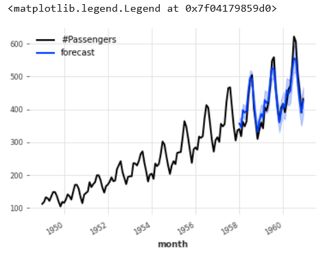
The monthly passenger values after 1960 seem to be forecasted with good accuracy due to model exponential smoothing as visible from the above plot.

3)  Kats

Kats (Kits to Analyze Time Series) is an open-source Python library developed by researchers at Facebook (now Meta). This library is easy to use and is helpful for time series problems. This is due to its very light weighted library of generic time series analysis which allows to set up the models quicker without spending so much time processing time series and calculations in different models.

Some significant features of the Kats library are –

• It works well for univariate and multivariate analysis.
• It can be used to perform forecasting with the available 10+ forecasting models.
• It handles outliers and can identify patterns, seasonality, and trends. Hence, it can be used for anomaly detection.
• It can be used for feature extraction and embedding with other machine learning models.

We can install this package using the following command-

pip install kats

Next, we import the necessary modules for the time series analysis

from kats.consts import TimeSeriesData
from kats.models.prophet import ProphetModel, ProphetParams
data.columns = ['month','#Passengers']
data['month'] = pd.to_datetime(data['month'],infer_datetime_format=True,format='%y%m')
df_s = TimeSeriesData(time=data['month'], value=data['#Passengers'])
df_s

# create a model param instance
params = ProphetParams(seasonality_mode='multiplicative')
# create a prophet model instance
model = ProphetModel(df_s, params)
# fit model simply by calling m.fit()
model.fit()
# make prediction for next 30 month
forecast = model.predict(steps=30, freq="MS")
forecast.head()

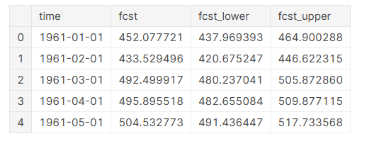
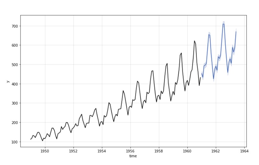
We can plot the forecast as

model.plot()

4) GreyKite

GreyKite is a time-series forecasting library released by LinkedIn to simplify prediction for data scientists. This library offers automation in forecasting tasks using the primary forecasting algorithm ‘Silverkite.’ This library also helps interpret outputs making it a go-to tool for most time-series forecasting projects.

A few interesting features of GreyKite are-

• It can perform exploratory data analysis (EDA), forecast pipeline, model tuning, benchmarking, etc.
• It can be used for feature engineering, anomaly detection, seasonality, etc.
• The Silverkite model offers several pre-tuned templates to fit different forecast frequencies, horizons, and data patterns.
• There is also an interface for the Prophet model developed by Facebook.

To install GreyKite, use the pip command-

pip install greykite

Next, we will set up the model using the following commands

from greykite.framework.templates.autogen.forecast_config import ForecastConfig
from greykite.framework.templates.autogen.forecast_config import MetadataParam
from greykite.framework.templates.forecaster import Forecaster 
from greykite.framework.templates.model_templates import ModelTemplateEnum
from greykite.framework.utils.result_summary import summarize_grid_search_results
# Specifies dataset information
metadata = MetadataParam(
     time_col="month",  # name of the time column
     value_col="#Passengers",  # name of the value column
     freq="MS"  #"MS" for Montly at start date
 )
forecaster = Forecaster()
result = forecaster.run_forecast_config(
     df=data,
     config=ForecastConfig(
         model_template=ModelTemplateEnum.SILVERKITE.name,
         forecast_horizon=100,  # forecasts 100 steps ahead
         coverage=0.95,  # 95% prediction intervals
         metadata_param=metadata
    )
)

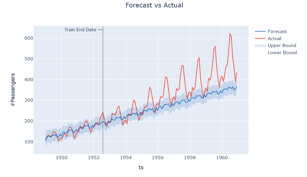
We can now plot the forecasted values as-

ts = result.timeseries
fig = ts.plot()
plotly.io.show(fig)

5) AutoTS

AutoTS, another Python time series tool, stands for Automatic Time Series, quickly providing high-accuracy forecasts at scale. It offers many different forecasting models and functions directly compatible with pandas’ data frames. The models from this library can be used for deployment. Some noticeable features of this library are –

• Works well with both univariate and multivariate time series data
• Can handle missing or messy data with outliers
• helps to identify the best time series forecasting model based on the input data type

Let us explore the applicability of this library to make a temperature prediction for the next month.

First, install the ‘autots’ package using the following lines of code:

pip install autots

Next, we will import the package

# Loading the package
from autots import AutoTS

We will use the previously imported dataset for Air passengers. We will create a TimeSeries object from a Pandas DataFrame and split it into a train/validation series.

from autots import AutoTS
model = AutoTS(forecast_length=12, frequency='infer',ensemble='simple')
model = model.fit(data, date_col='month', value_col='#Passengers', id_col=None)
prediction = model.predict()
#make predictions
forecast = prediction.forecast
print("Passengers Forecast")
print(forecast)

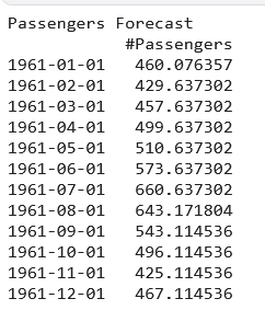
Next, we use the plt.show() command to visualize the predictions.

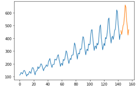
The AutoTS library seems to have predicted the passenger numbers well based on the existing patterns in the dataset.

Conclusion on Time-Series

There are many other popular libraries like Prophet, Sktime, Arrow, Pastas, Featuretools, etc., which can also be used for time-series analysis. In this article, we explored 5 Python libraries – Tsfresh, Darts, Kats, GreyKite, and AutoTS developed especially for Time-series analysis. Before closing this article, let us recap some crucial points.

Key takeaways From this Article:

• Time-series analysis can significantly impact the decision-making in a business or a real-world challenge.
• There are several open-source Python packages that Data Scientists across different organizations use to analyze real-world data and make future predictions. Choosing a library for a particular task depends on the project requirements and the preference of the Data Scientist implementing it.
• Implementing time-series analysis in these libraries requires a few lines of code. However, it is expected to have a good understanding of time-series concepts and make correct use of the results in decision-making.

I hope you enjoyed exploring these time-series libraries mentioned here in this article. Even if you might have used one of these for your past projects, try an alternate library from this list and have fun comparing the results. And if you haven’t tried any of these libraries, pick any one tool to get started. They are easy to implement but remember to read some time-series theory beforehand to better utilize these libraries for your project. You can find the code for this article on my GitHub repository.

The media shown in this article is not owned by Analytics Vidhya and is used at the Author’s discretion.

Devashree

Devashree has an M.Eng degree in Information Technology from Germany and a Data Science background. As an Engineer, she enjoys working with numbers and uncovering hidden insights in diverse datasets from different sectors to build beautiful visualizations to try and solve interesting real-world machine learning problems.

In her spare time, she loves to cook, read & write, discover new Python-Machine Learning libraries or participate in coding competitions.