This article was published as a part of the Data Science Blogathon.
Introduction
In this article, we will be discussing the binomial distribution where along with the theoretical knowledge of this particular distribution we will also see the practical implementation of the same for that we have to perform an experiment of flipping the coin and in this experiment, we will take two situations which are biased and unbiased condition.
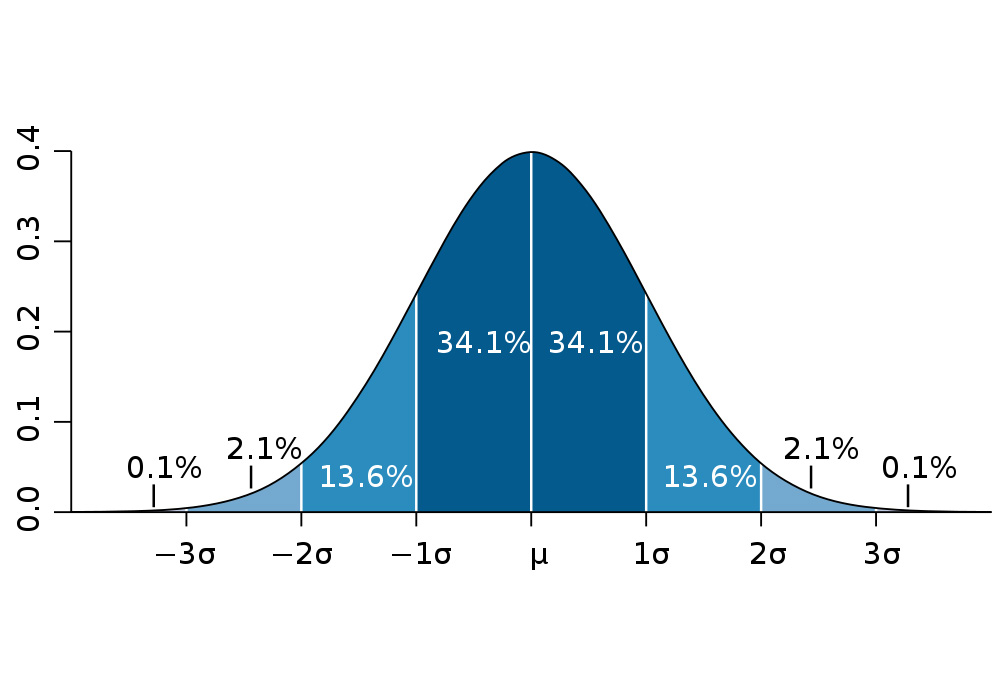
Probability Distribution in Statistics
Before moving to the main thing i.e. binomial distribution let’s discuss the background of probability distribution in statistics and its typed and for that let’s have a question and answer segment.
What does the term probability distribution mean?
If you are hearing any term for the first time just keep in mind to break it down and get whatever insight you can, here if we will break it down so it has possibility and distribution which resembles “Distributing all the possible/valid values according to the chances of their occurrence for a selected random variable”. By doing this we will get the range of values which will have the maximum and the minimum value and along with that, it will be dependent on various factors like skewness, standard deviation, kurtosis, etc.
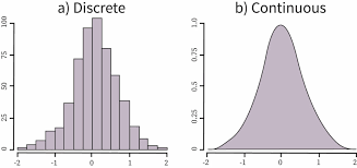
What are the types of the probability distribution?
So the distribution is divided into two main parts:
- Discrete Probability Distributions: This segment of the distribution signifies how many times a discrete random value has occurred in a graphical structure when we will plot it.
- Continuous Probability Distributions: Similarly this segment signifies how many times a continuous random variable has occurred in a graph.
Importing Statistics Package
Here we will be importing all the required packages which will involve doing the calculation stuff of all the statistics concepts and visualization of the distribution.
%matplotlib inline

import numpy as np
import pandas as pd
import matplotlib.pyplot as plt
import SCIPY.stats as stats
The Binomial Distribution
Binomial is one of the kinds of discrete distribution which simplifies one thing accurately i.e. it works on the discrete random variables and if we go through the typical definitions of binomial then it demonstrates that this kind of distribution of variables deals with the binary scenarios i.e. it will take the two independent values under the specified number of parameters with valid values of params to draw the plot based on the all the data points it considered after performing a certain number of trials.
What kind of trials does it perform?
Here, it performs the trials named Bernoulli trials, and to go with it we have to meet certain criteria and they are:
- There should always be only 2 possible outcomes that fulfill the criteria of binary scenarios
- Every happening trial should be completely independent of other trials which are already occurred or are yet to occur.
- Each outcome should occur i.e. there should be a fixed likelihood of the outcome to take place in an experiment.
Binomial function in python has three parameters to deal with and they are as follows:
- n: This value denotes the number of trials that need to occur in an experiment.
- p: This indicates the likelihood of the occurrence that will happen after each trial, we can take an example of tossing a coin where it has the occurrence as 0.5 for each.
- shape: This is responsible for how the shape should be of an array after a successful trial.
Experiment with the Binomial Distribution
In this section, we will be using python’s statistics packages to perform these distribution functions and visualize the same in this way we will not only be going through the theoretical part of it but able to understand the application of the real world and get to know about business-related use cases.

Image Source: National Today
Experiment
In this experiment, we are taking the famous flipping the coin example where we will be flipping the fair coin 10 times ( this can be denoted as several trials) and in this particular trial, we will change the occurrence of success to see the changes in the histograms (denoted as success probability which we say the likelihood of the occurred event) and also the number of trials.
What this experiment will tell us?
So here this question means what conclusions we can draw after the experiment that is performed so it will tell us when it is likely to get either 1 head or 2 head or 3 head or even 0 head and so on.
Binom() Function
So why we are using Python as we know we have the formula for binomial distribution so we can easily put values in it and implement the same but it becomes a very tedious task to follow on such complex calculations for that reason the SCIPY package of python have a reserve of almost all the statistics packages similarly it have the binomial function in the stats class.
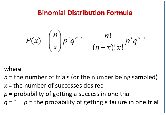
About binomial function
The “binomial()” function in the SCIPY package just needs three valid parameters values to give us the binomial distribution of all the values which were specified in several trials
Note: The parameters it needs are the same as those I discussed previously.
fair_coin_flips = stats.binom.rvs(n=10,
                                  p=0.5,
                                  size=10000)

print(pd.crosstab(index="counts", columns= fair_coin_flips))
Output:
col_0   0   1    2     3     4     5     6     7    8   9   10
row_0
counts   9  93  435  1200  2052  2419  2041  1212  439  90  10
Code breakdown
- Here firstly we are accessing the venom’s “RVS” function from the SCIPY’s stats package and then we are giving the value of the parameter is:
- n = 10 i.e. Total number of flips likely to occur or trial
- p = 0.5 i.e. occurrence of each event i.e. success probability
- size = 10000 i.e. total number of trials in an experiment.
- Then with the help of the crosstab function of pandas, we are getting the DataFrame which has counts and the number of coin flips from 1 to 10
Plotting the results
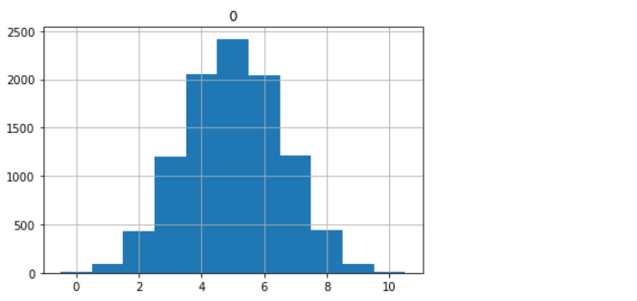
In this sub-section, we will plot the values that we got after performing the complete experiment of flipping the Fair coins here I’m mentioning the fair coins as the p-value is 0.5 which is an unbiased probability value in the next section we will also discuss unbiased distribution.
pd.DataFrame(fair_coin_flips).hist(range=(-0.5,10.5), bins=11)
Output:
array([[]], dtype=object)
Inference
In the above output, we can see that this plot demonstrates the “symmetric” graph and it shows us the 50% of the success probability with most of the outcomes that have occurred in the trials being situated in the center
Note: As we are well aware of the fact that binomial distribution belongs to the discrete part hence it can only hold up the integer values for that reason we can express these values as the frequency table and for its distribution, we can use the histogram
Biased condition
Now let’s change the success probability value from 0.5 to 0.8 – Biased condition of flipping the coin experiment. In this section, just after changing the value to 0.8, we will realize that it will be turned out to be a biased condition and which will be reflected in the values of the frequency table and histogram as well.
biased_coin_flips = stats.binom.rvs(n=10,
                                  p=0.8,
                                  size=10000)

# Printing the frequency table of counts
print(pd.crosstab(index="counts", columns= biased_coin_flips))
Output:
col_0   3   4    5    6     7     8     9     10
row_0
counts   2  51  274  859  2004  3113  2611  1086
Code breakdown:
Code explanation is the same as we have discussed previously just a change is in the value of success probability to 0.8 to determine and test the biased condition.
# Plot the histogram of the above frequency table
PD.DataFrame(biased_coin_flips).hist(range=(-0.5,10.5), bins=11);
Output:
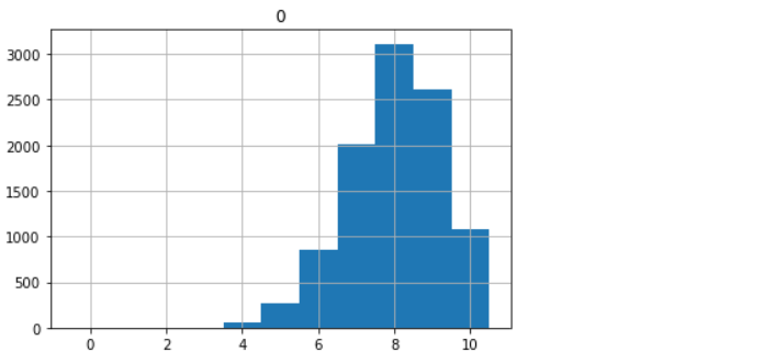
Inference: If we will compare the above-biased condition plot and the previous unbiased condition plot then we can surely spot the difference in this first condition i.e. unbiased one has the symmetric distribution most of the data points from the frequency table were situated in the center while the other one has the skewed structure i.e. non-symmetric and in this plot, we can see most of the data points are shifted to the right corner of the plot.
Note: Such plots are regarded as the “right-skewed” distribution.
Conclusion
In this article, we have discussed everything one needs to know about the binomial distribution from learning about the theoretical part of it to experiment with flipping the coin and traversing through both the condition of that experiment.
- Firstly, we laid the foundation for understanding the terms of distribution in statistics and its types.
- Then we move specifically toward the binomial distribution and learned about it and its function and parameters.
- Then at the last for practical knowledge, we performed an experiment that helped us to visualize the results and helped us to understand this distribution more perfectly.
Here’s the repo link to this article. I hope you liked my article on reversing the video using computer vision. If you have any opinions or questions, then comment below.
Connect with me on LinkedIn for further discussion.
The media shown in this article is not owned by Analytics Vidhya and is used at the Author’s discretion.


in a biased condition , i think it became left skewed , kindly check and correct me if i'm wrong.