Handling Missing Values with Random Forest

Introduction to Random Forest

Missing values have always been a concern for any statistical analysis. They significantly reduce the study’s statistical powers, which may lead to faulty conclusions. Most of the algorithms used in statistical modellings such as Linear regression, Logistic Regression, SVM and even Neural Networks are prone to these missing values. So, knowledge of handling lost data is a must. Several methods are popularly used to manage missing data. This article will discuss the Random Forest method of filling missing values and see how it fares compared to another popular technique, K-Nearest Neighbour.

What are the Missing Data?

Missing data is the data value not stored for a variable in the observation of interest. There are four ways the missing values could occur in a dataset. And those are

• Structurally missing data,
• MCAR(missing completely at random),
• MAR(Missing at random) and
• NMAR(Not missing at random).

Structurally missing data: These are missing because they are not supposed to exist. For example, the age of the youngest kid of a couple having no kids is best addressed by excluding the observations from any analysis of the variables.

 MCAR (Missing Completely At Random): These are the missing values that occur entirely at random. There is no pattern, and each missing value is unrelated. For example, a weighing machine that ran out of batteries. Some of the data will be lost just because of bad luck, and the probability of each missing data is the same throughout.

MAR (Missing At Random): The assumption here is that the missing values are somewhat related to the other observations in the data. We can predict the missing values by using information from other variables, such as indicating a person’s missing height value from age, gender, and weight. This can be handled using specific imputation techniques or any sophisticated statistical analysis.

NMAR(Not Missing At Random): If the data cannot be classified under the above three, the missing value falls in this category. The missing values here originated not at random but deliberately. For example, people in a survey slowly do not answer some questions.

Imputation Techniques

There are many imputation techniques we can employ to tackle missing values. For example, imputing means for continuous data is the most routine matter in the case of categorical data. Or we can use machine learning algorithms like KNN and Random Forests to address the missing data problems. For this article, we will be discussing Random Forest methods, Miss Forest, and Mice Forest to handle missing values and compare them with the KNN imputation method.

Random Forest for Missing Values

Random Forest for data imputation is an exciting and efficient way of imputation, and it has almost every quality of being the best imputation technique. The Random Forests are pretty capable of scaling to significant data settings, and these are robust to the non-linearity of data and can handle outliers. Random Forests can hold mixed-type of data ( both numerical and categorical). On top of that, they have a built-in feature selection technique. These distinctive qualities of Random Forests can easily give it an upper hand over KNN or any other methods.

KNN, on the other hand, involves the calculation of Euclidean distance of data points, thus making it prone to outliers. It cannot handle categorical data, so data transformation is needed, and it requires the data to be scaled to perform better. All these things can be bypassed by using Random Forest-based imputation methods.

For this article, we will discuss two such methods: Miss Forest and the other is Mice Forest. We will explore how they work and their python implementation.

Miss Forest

Arguably the best imputation method. If you need precision, then this is what you must use. An iterative imputation technique powered by Random Forest to precisely impute data. So, how does it work?

Step-1: First, the missing values are filled by the mean of respective columns for continuous and most frequent data for categorical data.

Step-2: The dataset is divided into two parts: training data consisting of the observed variables and the other is missing data used for prediction. These training and prediction sets are then fed to Random Forest, and subsequently, the predicted data is imputed at appropriate places. After imputing all the values, one iteration gets completed.

Step-3: The above step is repeated until a stopping condition is reached. The iteration process ensures the algorithm operates on better quality data in subsequent iterations. The process continues until the sum of squared differences between the current and previous imputation increases or a specific iteration limit is reached. Usually, it takes 5-6 iterations to attribute the data well.

Source: Andre Ye

Advantages of Missing Forest

There are several advantages to using Missing Forest for imputation.

• It can work with mixed data, both numerical and categorical
• Miss Forest can handle outliers, so there is no need for feature scaling.
• Random Forests have inherent feature selection, which makes them robust to noisy data.
• It can handle non-linearity in data

Disadvantages of Missing Forest

• Multiple trees need to be constructed for each iteration, and it becomes computationally expensive when the number of predictors and observations increases.
• Also, it’s an algorithm, not a model object, meaning it must be run every time data is imputed, which could be problematic in some production environments.

Mice Forest

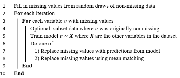
Another interesting imputation method is the Mice algorithm stands for Multiple Imputation By Chained Equation. Technically any predictive model can be used with mice for imputation. Here we will be using LIghtGBM for prediction. And this is more or less similar to miss forest as far as pseudocode of algorithm is involved. The only difference in the package we will be dealing with is it uses a LightGBM instead of a  pure Random Forest.  The pseudocode for the algorithm is given as

More on this you can find here.

Python Example

The best way to show the efficacy of the imputers is to take a complete dataset without any missing values. And then amputate the data at random and create missing values. Then use the imputers to predict missing data and compare it to the original.

For this section, we will also be using the KNN imputation method to give a performance comparison between them.

Import Libraries

Before going further, we would like to install several packages that we will be using further. We will use the missingpy library for Miss Forest, while we will use the Mice Forest for Mice Forest.

!pip install missingpy
!pip install miceforest

Now, we will import libraries.

import pandas as pd
import numpy as np
import matplotlib.pyplot as plt
import seaborn as sns
import miceforest as mf
import random
import sklearn.neighbors._base 
import sys
sys.modules['sklearn.neighbors.base'] = sklearn.neighbors._base
from missingpy import MissForest
from sklearn.impute import KNNImputer

For this article, we will be using the California Housing dataset.

from sklearn.datasets import fetch_california_housing

Convert it to workable pandas data frame format

Python Code:

import pandas as pd
import numpy as np
import matplotlib.pyplot as plt
import seaborn as sns
import miceforest as mf
import random
import sklearn.neighbors._base 
import sys
sys.modules['sklearn.neighbors.base'] = sklearn.neighbors._base
from missingpy import MissForest
from sklearn.impute import KNNImputer
from sklearn.datasets import fetch_california_housing

df2 = pd.concat(fetch_california_housing(return_X_y=True, as_frame=True),axis=1)
df2 = df2.copy()
print(df2.head())

Amputation for Random Forest

We will now introduce nan values at random in the dataset.

r1 = random.sample(range(len(df2)),36)
r2 = random.sample(range(len(df2)),34)
r3 = random.sample(range(len(df2)),37)
r4 = random.sample(range(len(df2)),30)
df2['AveRooms'] = [val if i not in r1 else np.nan for i, val in enumerate(dt2['AveRooms'])]
df2['HouseAge'] = [val if i not in r2 else np.nan for i, val in enumerate(dt2['HouseAge'])]
df2['MedHouseVal'] = [val if i not in r3 else np.nan for i, val in enumerate(dt2['MedHouseVal'])]
df2['Latitude'] =    [val if i not in r4 else np.nan for i, val in enumerate(dt2['Latitude'])]

Imputation for Random Forest

Now, we will use each of the three techniques to impute data.

# Create kernels.  #mice forest
kernel = mf.ImputationKernel(
  data=df2,
  save_all_iterations=True,
  random_state=1343
)
# Run the MICE algorithm for 3 iterations on each of the datasets
kernel.mice(3,verbose=True)
#print(kernel)
completed_dataset = kernel.complete_data(dataset=0, inplace=False)

imputer = MissForest() #miss forest
X_imputed = imputer.fit_transform(df2)
X_imputed = pd.DataFrame(X_imputed, columns = df2.columns).round(1)

Knn Imputation

impute = KNNImputer() #KNN imputation
KNNImputed = impute.fit_transform(df2)
KNNImputed = pd.DataFrame(KNNImputed, columns = df2.columns).round(1)

Evaluation

To evaluate the outcomes of the results, we will use the sum of the absolute differences between the imputed dataset and the original dataset. Only the columns and rows with null values will be used here, and this is to get an overall idea of the efficiency of the model.

missF = np.sum(np.abs(X_imputed[df2.isnull().any(axis=1)] -         dt2[df2.isnull().any(axis=1)]))
mice =  np.sum(np.abs(completed_dataset[df2.isnull().any(axis=1)] - dt2[df2.isnull().any(axis=1)]))
Knn =   np.sum(np.abs(KNNImputed[df2.isnull().any(axis=1)] -        dt2[df2.isnull().any(axis=1)]))
for i in [missF, mice, Knn]:
    print(np.sum(i))

output:274.3717058165446
361.4645867313583
497.2673601714581

From the above outcome, we can have a rough estimate of the efficacy of each method, and it seems Miss Forest was able to recreate the original model better, followed by Mice Forest and then KNN.

We didn’t do any feature transformation, which means KNN, which relies on euclidean distance, suffered a lot.

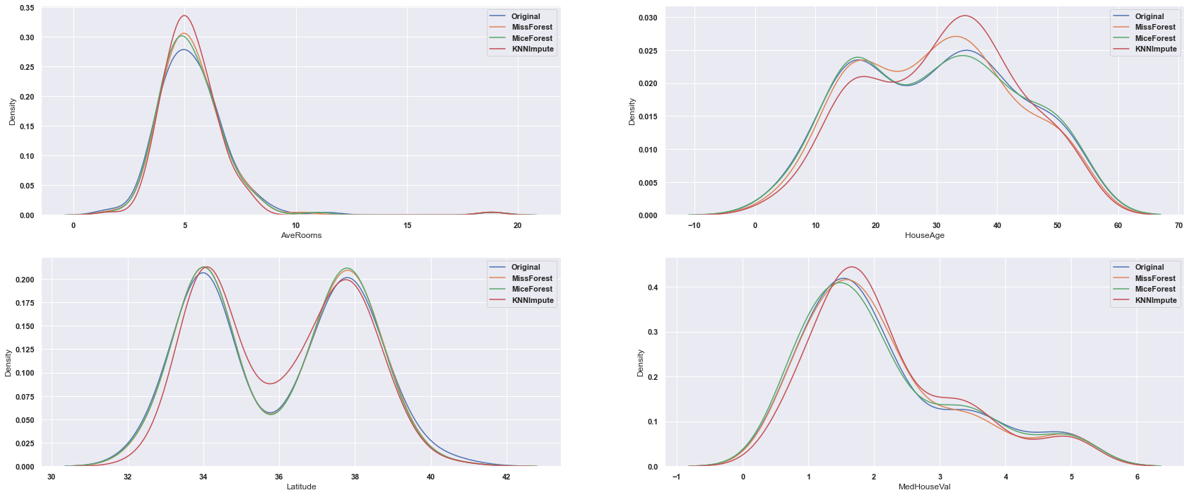
We can also visualize the same using Seaborn and Matplotlib.

sns.set(style='darkgrid')
fig,ax = plt.subplots(figsize=(29,12),nrows=2, ncols=2)
for col,i,j in zip(['AveRooms','HouseAge', 'Latitude','MedHouseVal'],[0,0,1,1],[0,1,0,1]):
    sns.kdeplot(x = dt2[col][df2.isnull().any(axis=1)], label= 'Original', ax=ax[i][j] )
    sns.kdeplot(x = X_imputed[col][df2.isnull().any(axis=1)], label = 'MissForest', ax=ax[i][j] )
    sns.kdeplot(x = completed_dataset[col][df2.isnull().any(axis=1)], label = 'MiceForest', ax=ax[i][j] )
    sns.kdeplot(x = KNNImputed[col][df2.isnull().any(axis=1)], label='KNNImpute',  ax=ax[i][j] )
    ax[i][j].legend()

The previous result can be verified here as Miss Forest traces closer to the original data, followed by the Mice Forest and then KNN.

This was a rough evaluation of the three imputation methods we used. Note: We didn’t take the bias introduced by each technique into account while evaluating. This is meant to give just a rough idea of imputation accuracy.

Conclusion

Missing values are nothing less than a headache. The data generated from real-world processes are even more prone to missing values. Knowing methods that can efficiently handle missing data is a must. This article highlighted the Random Forest methods for tackling missing data, their advantages, and their disadvantages. And finally, we compared these methods with the popular KNN imputation method. It is safer to say that Random Forest methods outperform other methods. Next time you encounter missing data, consider using these methods.

The media shown in this article is not owned by Analytics Vidhya and is used at the Author’s discretion. 

Sunil Kumar

Meet your author Sunil kumar Dash, a developer and a writer. Has diverse interests in tech, pop culture, wellness, philosophy and Anime. Exploring underrated music is his hobby. And loves to doom scroll Twitter when bored.