How to Approach CNN Architecture from Scratch?

This article was published as a part of the Data Science Blogathon.

Introduction on CNN Architecture

Hello, and welcome again to another intriguing subject. As a consequence of the large quantity of data accessible, particularly in the form of photographs and videos, the need for Deep Learning is growing by the day. Many advanced designs have been observed for diverse objectives, but Convolution Neural Network – Deep Learning techniques are the foundation for everything. So that’ll be the topic of today’s piece.

Deep Learning

Deep learning is a machine learning and artificial intelligence (AI) area that mimics how people learn. Data science, which covers statistics and predictive modeling, contains deep learning as a significant component. For data scientists who must obtain, analyze, and interpret massive volumes of data, deep learning is particularly useful since it speeds up and simplifies the process.

Layman’s Explanation of Deep Learning

I hope you all enjoyed Inception (2010), a film with an idea and technology application that is both baffling and exciting. The film’s major theme is that a dream may be used to implant a thought in a person’s subconscious mind, which subsequently influences their behavior. This may be accomplished through the use of a creative notion known as shared dreaming. This is what “deep learning” implies simply put (Inception on a Machine rather than a person)

Using the above Inception timeline, you may need to go down several layers deep into the machine neural structure (technically called forward propagation, but in the diagram, it’s called the different level of dreams) and perform a kick (backpropagation) to reinforce the learning, depending on what you want to achieve. For inception, the neural nodes (shared-state dreamers) utilize an activation function/architect (Relu, Sigmoid, and others).

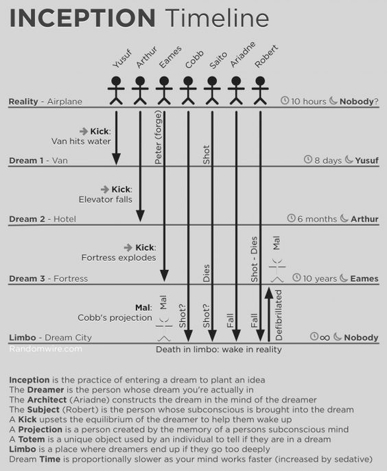
The nodes/people in the current layer (vanishing gradient) may be assassinated and go into limbo on rare occasions, jeopardizing the entire inception (learning) process. Fortunately, a skilled pharmacist (bias function / leaky Relu) may be able to provide the therapy needed to avoid it. It’s probable that you’ll have to perform this procedure (machine learning epoch) numerous times before you achieve convergence, which means the system is behaving as intended.

You’ll need a featured architect just like you’ll need an architect to design your beautiful landscape. As the genesis process goes, you seed the machine with a feature, and it continues to build more and more intricate features. From the input, each buried layer creates a feature. As you go through the phases, these features become more sophisticated and responsive to learning. As a result, you essentially produce conception by probing deep into the machine’s psyche. The system then “learns” to recognize faces, handwriting, optical characters, and other unimaginable objects.

Why do we go from Machine Learning to Deep Learning?

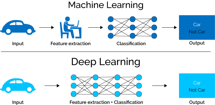
The bulk of the necessary features in Machine Learning approaches must be determined by a domain expert to reduce data complexity and make patterns more obvious for learning algorithms to work. The main advantage of Deep Learning algorithms is that they seek to gain high-level qualities from data progressively. As a result, the requirement for domain expertise and the extraction of hard-core features is decreased.

Deep Learning approaches need to break down problem statements into different pieces and then combine their results at the conclusion, whereas Machine Learning strategies require breaking down problem statements into distinct parts and then combining their results at the end. Deep learning systems like Yolo net take a photo as input and output the position and names of objects in a multiple object detection task. However, before the HOG can be used as an input to a learning algorithm to categorize relevant items in Machine Learning methods like SVM, it must first be used to identify all conceivable objects using a bounding box object identification approach.

Types of Deep Learning

There are many types based on application and the architecture,

1. Artificial Neural Network
2. Convolution Neural Network
3. Recurrent Neural Network
4. Autoencoders
5. Self Organizing Map
6. Multi-layer Perceptron and many more…

Convolution Neural Network:

In simple, A convolutional neural network is a deep learning network design that learns from the input without the requirement for human feature extraction. Please refer to this blog for a detailed explanation

Layers in Convolution Neural Network

CNN has certain building components for constructing the architecture, such as

Convolution layer

The convolutional layer, which holds the majority of the computation, is the foundation of a CNN. It requires input data, a filter, and a feature map, among other things. Assume the input is a 3D pixel matrix with a color picture. This implies that the input will have three dimensions that correspond to an image’s RGB color space. A feature detector, also known as a kernel or a filter, will look for the feature in the image’s receptive fields. Convolution is the name for this technique.

When the filters don’t fit the input image, zero padding is utilized. All members are set to zero outside of the input matrix, resulting in a bigger or comparable output. Padding comes in three varieties:

No Valid padding is also known as valid padding. If the dimensions do not align, the final convolution is discarded.

Same Padding: This padding guarantees that the output layer matches the input layer in size.

Full Padding: By padding, the input with zeros, this form of padding increases the size of the output.

Activation layer

To determine whether a neuron should be activated or not, the activation function produces a weighted sum and then adds bias to it. The activation function’s purpose is to make a neuron’s output non-linear.

Pooling layer

The number of parameters in input is reduced using a dimensionality reduction technique called a pooling layer or downsampling. The pooling approach, like the convolutional layer, sweeps a filter across the whole input, but this filter does not include any weights. Instead, the kernel uses an aggregation function to fill the output array with values from the receptive field.

Max pooling: The filter picks the pixel with the highest value to transmit to the output array as it advances across the input. In comparison to average pooling, this strategy is employed more frequently.

Average pooling: The filter calculates the average value inside the receptive field as it passes across the input and sends it to the output array.

Flattening and Fully Connected Network 

A convolutional neural network’s last level is a classifier (CNN). It’s called a dense layer, and it’s just an artificial neural network (ANN) classifier.

An ANN classifier, like any other classifier, requires certain properties. This suggests that a feature vector is required.

As a result, you must convert the output of the convolutional component of the CNN into a 1D feature vector that the ANN can use. This procedure is known as flattening. It flattens all of the structure of the convolutional layers’ output into a single long feature vector that the dense layer may use for classification.

Advantages

1. Better to train the model in terms of computing
2. Very High accuracy in image recognition problems
3. Automatically detects the important features without any human supervision.

Disadvantages

1. Adversarial attacks
2. Data-intensive training

Applications of CNN

1. Image classification
2. Object detection
3. Audiovisual matching
4. Object reconstruction
5. Speech recognition

CNN Using Image

Original Dataset

Kaggle Dataset

!wget https://download.microsoft.com/download/3/E/1/3E1C3F21-ECDB-4869-8368-6DEBA77B919F/kagglecatsanddogs_3367a.zip

#for unzipping the dataset
!unzip kagglecatsanddogs_3367a.zip

after we download the necessary dataset that we need for processing, we need to import some basic libraries,

import numpy as np
import pandas as pd
import matplotlib.pyplot as plt
from keras.preprocessing.image import load_img
import warnings
import seaborn as sns
import os
import random
warnings.filterwarnings('ignore')

all the images in the file can be converted to data frame format for further process to make it smooth,

#Cat - 0 and Dog -1

input_path = []
label = []

for class_name in os.listdir("PetImages"):
    for path in os.listdir("PetImages/"+class_name):
        if class_name == 'Cat':
            label.append(0)
        else:
            label.append(1)
        input_path.append(os.path.join("PetImages", class_name, path))
print(input_path[20000], label[20000])

to cross-check and see the result,

print(input_path[2], label[2])

some basic statistical and view the dataset,

len(input_path)
dataset = pd.DataFrame()
dataset['images'] = input_path
dataset['label'] = label
dataset = dataset.sample(frac=1).reset_index(drop=True)
dataset.head()
dataset.tail()
dataset.shape
dataset.info()

in order to delete the junk or useless files other than the .jpg format

#for corrupted images
import PIL
l = []
for image in dataset['images']:
    try:
        img = PIL.Image.open(image)
    except:
        l.append(image)
l

deleting the above mentioned unwanted files

# delete db files
dataset = dataset[dataset['images']!='PetImages/Dog/Thumbs.db']
dataset = dataset[dataset['images']!='PetImages/Cat/Thumbs.db']
dataset = dataset[dataset['images']!='PetImages/Cat/666.jpg']
dataset = dataset[dataset['images']!='PetImages/Dog/11702.jpg']
len(dataset)

EDA – Dog

# to display grid of images
plt.figure(figsize=(25,25))
temp = dataset[dataset['label']==1]['images']
start = random.randint(0, len(temp))
files = temp[start:start+25]

for index, file in enumerate(files):
    plt.subplot(5,5, index+1)
    img = load_img(file)
    img = np.array(img)
    plt.imshow(img)
    plt.title('Sample Dogs images')
    plt.axis('off')

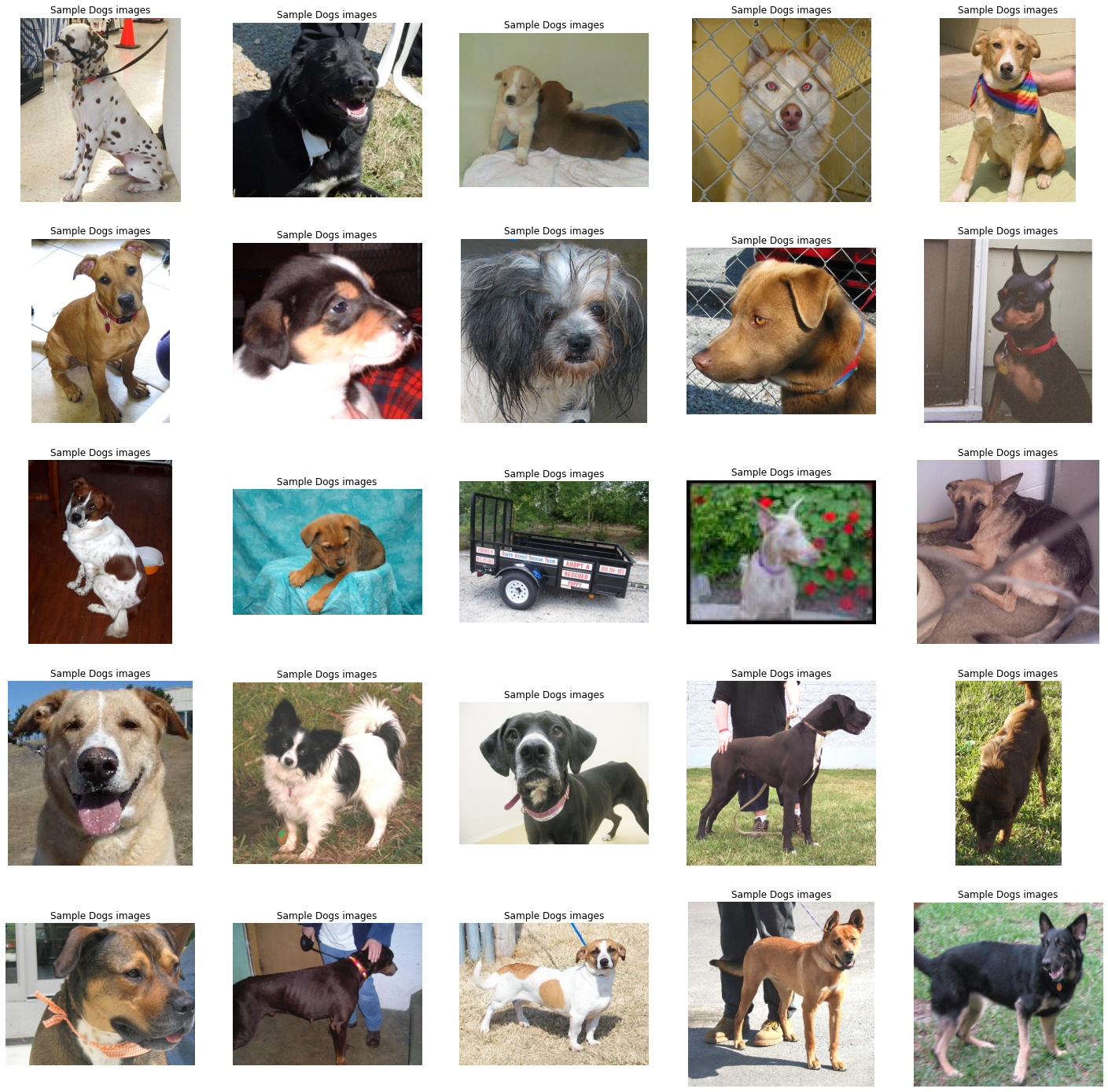
EDA – Cat

# to display grid of images
plt.figure(figsize=(25,25))
temp = dataset[dataset['label']==0]['images']
start = random.randint(0, len(temp))
files = temp[start:start+25]

for index, file in enumerate(files):
    plt.subplot(5,5, index+1)
    img = load_img(file)
    img = np.array(img)
    plt.imshow(img)
    plt.title('Sample Cats images')
    plt.axis('off')

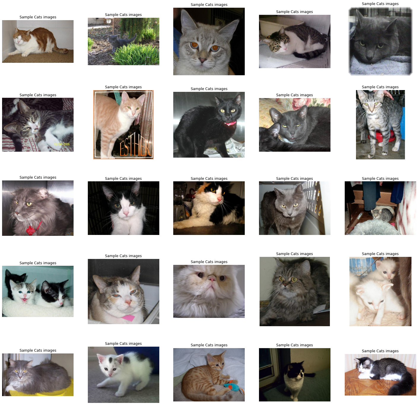
as both the category which has an equal amount of data,

sns.countplot(dataset['label'])

Datagenertor for Images

dataset['label'] = dataset['label'].astype('str')

# input split
from sklearn.model_selection import train_test_split
train, test = train_test_split(dataset, test_size=0.3, random_state=42)
from keras.preprocessing.image import ImageDataGenerator
train_generator = ImageDataGenerator(
    rescale = 1./255,  # normalization of images
    rotation_range = 40, # augmention of images to avoid overfitting
    shear_range = 0.2,
    zoom_range = 0.2,
    horizontal_flip = True,
    fill_mode = 'nearest'
)

val_generator = ImageDataGenerator(rescale = 1./255)

train_iterator = train_generator.flow_from_dataframe(
    train, 
    x_col='images', 
    y_col='label', 
    target_size=(128,128), 
    batch_size=512, 
    class_mode='binary'
)
val_iterator = val_generator.flow_from_dataframe(
test,
x_col='images',
y_col='label',
target_size=(128,128),
batch_size=512,
class_mode='binary'
)

Modeling

from keras import Sequential
from keras.layers import Conv2D, MaxPool2D, Flatten, Dense

model = Sequential([
                    Conv2D(16, (3,3), activation='relu', input_shape=(128,128,3)),
                    MaxPool2D((2,2)),
                    Conv2D(32, (3,3), activation='relu'),
                    MaxPool2D((2,2)),
                    Conv2D(64, (3,3), activation='relu'),
                    MaxPool2D((2,2)),
                    Conv2D(128, (3,3), activation='relu'),
                    MaxPool2D((2,2)),
                    Flatten(),
                    Dense(256, activation='relu'),
                    Dense(1, activation='sigmoid')
])

model.compile(optimizer='adam', loss='binary_crossentropy', metrics=['accuracy'])
model.summary()

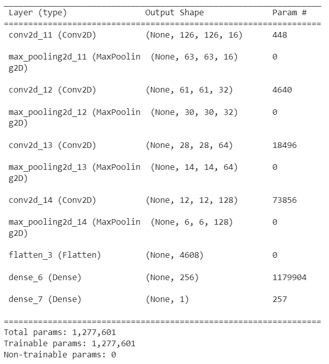
history = model.fit(train_iterator, epochs=15, validation_data=val_iterator)

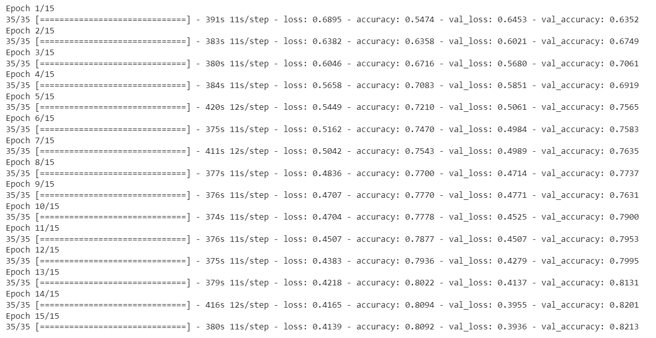
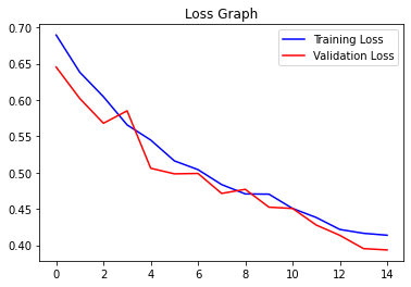
In order to see the output in visualization

acc = history.history['accuracy']
val_acc = history.history['val_accuracy']
epochs = range(len(acc))
plt.plot(epochs, acc, 'b', label='Training Accuracy')
plt.plot(epochs, val_acc, 'r', label='Validation Accuracy')
plt.title('Accuracy Graph')
plt.legend()
plt.figure()
loss = history.history['loss']
val_loss = history.history['val_loss']
plt.plot(epochs, loss, 'b', label='Training Loss')
plt.plot(epochs, val_loss, 'r', label='Validation Loss')
plt.title('Loss Graph')
plt.legend()
plt.show()

Conclusion

We’ve come to the end of the topic, so the main takeaways are, that we have seen how we are getting datasets from websites, then what are the basic preprocessing or data argumentation is needed for any basic image processing, and then we are constructing CNN architectures using layers like convolution, maxpool, flatten and dense layers. The reason for this blog is, that we have to understand the basic architectures, which leads to advanced architectures like GAN, YOLO, etc.

The media shown in this article is not owned by Analytics Vidhya and is used at the Author’s discretion.

Premanand S

Premanand S is a dedicated academic with over a decade of research experience, specializing in Bio-signal Processing, Machine Learning, and Deep Learning. He completed his B.Tech in 2009 from Amrita Vishwa Vidyapeetham, Bangalore, and his M.E. in 2011 from Rajalakshmi Engineering College, Chennai, where his thesis focused on Deep Learning for ECG Signal Processing.

He is pursuing his Ph.D. at VIT-Chennai, with a tentative research title of "Deep Learning Approaches for Enhanced ECG Signal Processing and Arrhythmia Classification." His research aims to leverage cutting-edge deep learning techniques to improve the accuracy and efficiency of ECG signal analysis, contributing significantly to cardiac health monitoring.

A recipient of the prestigious TCS-RSP (Research Scholarship) in 2014, Cycle 9, Premanand has become a recognized figure in the academic community. He has delivered several invited talks on Data Science, Machine Learning, and Deep Learning at prominent institutions across India.

In his role as an Assistant Professor at VIT-Chennai, he continues to inspire the next generation of researchers while advancing the boundaries of knowledge in his field.