Understanding Key Concepts on Data Warehouses

This article was published as a part of the Data Science Blogathon.

Introduction on Data Warehouses

During one of the technical webinars, it was highlighted where the transactional database was rendered no-operational bringing day to day operations to a standstill. The cause of the crash was attributed to the use of large-scale queries on the transactional database for which the design of the transactional database is not optimized. In the context of data engineering, the Data Warehouse is a critical Data Engineering asset to provide a data source for Business reporting tools like PowerBI to present the business analytics. This article is intended to look at concepts of DWH and highlight the same with some hands-on practice.

Data Warehouses

 

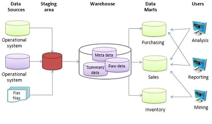
A sample data warehouse architecture is shown in the diagram The input data can come from multiple sources and they are extracted, transformed, and loaded(ETL process) into a Data Warehouse(DWH) using an ETL tool through an intermediate step called staging area. The structured data in DWH can be further used for analysis and reporting. In some use cases, the data from DWH is further segregated individually into a Data Mart which compartmentalizes the data used by specific users like Marketing, Sales, etc.

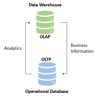
When we talk about databases for organizational requirements, we refer to Online Transactional Processing(OLTP) and Online Analysis Analytical Processing(OLAP). An OLTP system is designed to capture and maintain transaction data in a specific database. For example, a supermarket may use an application to capture the transaction during check out of goods at the counter. On the other hand, the OLAP database is designed to accept complex queries on large amounts of historical data to derive meaningful information for business analytics.

Data Warehouses Schema

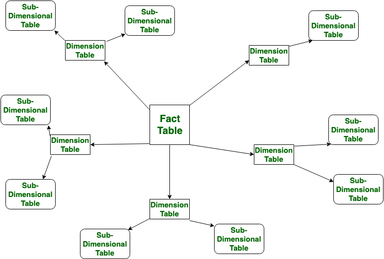
Data Warehouses schema is a logical description of the entire database. The Database designer creates a database schema to help developers who develop the application interact with the database tables. The process of creating a schema is called data modeling. Similar to a transactional database, the Data Warehouses schema also has a schema and three types of the Data Warehouses schema are seen here, viz, star, snowflake, and galaxy schema.

Star Schema

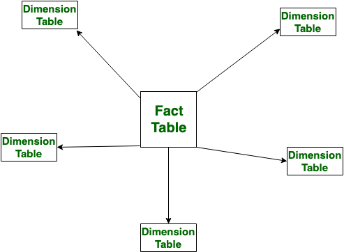
In star schema a fact table is located at the center of the schema and the dimensional tables branch off to form a star. The star schema is widely used for its simplistic design. The center table (fact) stores the specific quantifiable business data to be analyzed. For example, it could be sales data, financial data, etc. A sales data (say, a plain number of total sales is just a number and does not give much information) without context is just a number and does not provide actionable information. Dimension tables (also called reference tables) provides supporting information . A foreign key and primary key relationship connects the fact and dimension tables. As an example, a fact table contains sales data of a supermarket chain, and a store table (dimension) may store information containing store name, location, store manager, etc.

Snowflake Schema

]

Hands-on Exercise on Data Warehouses

Sometimes, a dose of too much theory can put the readers to sleep, hence we switch over to some hands-on practice to cement our learning of DWH concepts. Please feel free to read up more on the concepts highlighted above to strengthen the fundamentals.

Problem Description

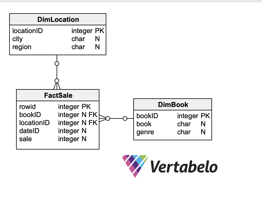
M/s ABC is a popular chain of bookstores in town. We have the transactional data of the number of sales of books at different stores which are spread out in cities and we need to design a DWH and load the data into the DWH for analysis and reporting. To keep it simple, the report the management is looking for is which books are sold maximum and the storewide sale of top books. The DWH schema has one facttable and two dimensiontables designed in a star schema. The fact table houses the data ( measure) of how many books are sold, and DimBook stores the information about the book (name and genre), and DimLocation stores data related to where the store is located(city and region).To keep the design simple the dimensiontable related to date has been left out .

Source Data

The input data is a CSV file(book_sale.csv) which contains the title and genre of books sold in stores and their numbers sold on a specific date. The look up table mapping the store to region is available in region.csv. We can go ahead and visualize the star schema for the DWH.

Target Data Warehouses

There are multiple options to create our target data warehouse One option is to use a cloud service provider like AWS, Google, Microsoft(Azure) , IBM etc. This is one of popular options for most enterprises unless the specific requirements demand a need to go for an on-premise data warehouse ( banks for example). I have opted for a simple PostgreSQL database running on a Docker container as our target data warehouse for the data pipeline.

Launching PostgreSQL Database in Docker

Docker is a tool that can be used to create, deploy and run applications in containers ( conceptually something similar to the one used on ships ). We can package and ship an application along with all the parts it needs like libraries and other dependencies . I am not focusing on the subject of docker in detail here for the fear of losing the focus on our data pipeline. Please feel free to look at my other articles in Analytics Vidhya or the information available in the internet to explore the subject of docker. The pre-requisites for going ahead with the hands-on exercise are the installation of the Docker Desktop and pgcli (CLI tool to access the Postgres database ). The relevant links are provided in the references section. Alternate tools like pgadmin, DBeaver, etc (GUI-based tools), can be used to interact with the database.

Assuming that Docker and pgcli have been successfully installed on the local machine, open the Terminal, navigate to your project directory and confirm the installation.

Create a folder in the project folder called sale_books_postgres_data . This folder will be mapped to the folder in the container for storage for persistent data.  The following command can be used to run PostgreSQL container on the terminal ,

docker run -it 
  -e POSTGRES_USER="root" 
  -e POSTGRES_PASSWORD="root" 
  -e POSTGRES_DB="sale_books" 
  -v $(pwd)/sale_books_postgres_data:/var/lib/postgresql/data 
  -p 5432:5432 
  postgres:13

The docker run command contains

• the docker image we are using is Postgres:13 (image is like a blueprint to create a container)
• docker run command gets the container running
• -it flag indicates the interactive mode of execution
• the name of our database is sale_books and the username and password are ‘root‘
• the volume mapping is done using the -v flag (use the full path of folder in case of windows os)
•  port 5432 on localhost has been mapped to port 5432 on the docker container

 

The above screen on running the docker run command shows the PostgreSQL database is ready . Open a new terminal and we can see run the following command

docker ps

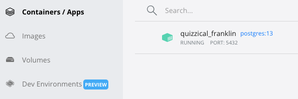
The above screenshots (one from the terminal and one from the Docker desktop application) indicate the container is running at port 5432 of the local machine and as we have not named the container specifically, the docker assigns a random name to the container. We can use pgcli from the terminal to connect to the database and explore further.

pgcli -h localhost -p 5432 -u root -d sale_books

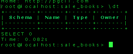
There are no tables created in our database yet and hence no tables are displayed. As an example the command ? displays all commands available. The link for pgcli commands is placed in the references section.

One approach we can use to create the star schema and corresponding tables in our sale_books database is using the pgcli (SQL commands). Another approach we can use is to create python scripts to create our schema and load the data into the tables thereby getting our DWH ready. In this exercise, we will use available python script to connect to the database and create our DWH.

Creating a Virtual Environment

Before we start writing our python script, it is a good practice to create a virtual environment for the project. A virtual environment is a tool for the developer which helps us to keep the dependencies required by one project separate from other projects by creating virtual environments for them. We can think of virtual environments similar to organized reference bookshelf for writing our book. If we are writing a book on politics then we do not need reference books on sports. Virtual environments help us to keep the packages we need for developing our application and also specify version of packages we want for our project. I have used conda to create the virtual environment for the project, there are tools like venv, virtualenv or pipenv to create the virtual environment.

Once you create a project directory, create a virtual environment within the project directory.

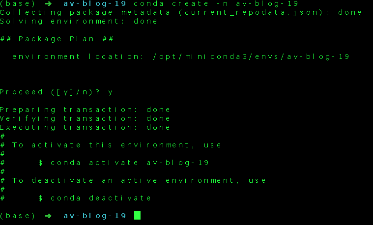
Now that the virtual environment is set up, we can install the libraries required for the project using the pip command

pip3 install pandas sqlachemy psycopg2+binary

The python script create_tables.py will create the tables and star schema in our database sale_books. The python script etl_dwh.py will create the ingestion script which takes the source data and populates the target tables in our DWH. A typical data pipeline to put data into DWH may usually involve a staging area. The staging area or landing zone is intermediate storage step generally used for data processing or transformation during the ETL(Extract Transform and Load) process. However, in the present exercise for the sake of simplicity, the staging area has not been used.

Create a file called config.py with following contents to store environment variables,

user = 'root'
password = 'root'
host = 'locahost'
port = "5432"
db="sale_books"

Create another file called create_tables.py

#importing necessary libraries
import pandas as pd
from sqlalchemy import create_engine
import psycopg2
#reading from config file
config = {}
exec(open('config.py').read(), config)
user = config['user']
password = config['password']
port = config['port']
db = config['db']

The above part of the code imports necessary libraries and also reads from config.py (please ensure the config.py is in the same project directory). The next step is to connect to the database  running on the localhost.

# Connect to the PostgreSQL database server
engine = create_engine(f'postgresql+psycopg2://{user}:{password}@localhost/{db}')
conn_string = f"host='localhost' dbname='{db}' user='{user}' password='{password}'"
conn = psycopg2.connect(conn_string)
# Get cursor object from the database connection
cursor = conn.cursor()

Using the cursor object we can run SQL queries inside the python script.

create_facttable = '''
CREATE TABLE public."FactSale"
(
    rowid integer NOT NULL,
    bookID INTEGER,
    locationID INTEGER,
    dateID INTEGER,
    sale INTEGER,
    PRIMARY KEY (rowid)
);'''
create_dimlocation = '''
CREATE TABLE public."DimLocation"
(
    locationID integer NOT NULL,
    city CHAR,
    region CHAR ,
    PRIMARY KEY (locationID)
);'''
create_dimbook = '''
CREATE TABLE public."DimBook"
(
    bookID integer NOT NULL,
    book CHAR,
    genre CHAR ,
    PRIMARY KEY (bookID)
);'''

# execute sql queries to create tables and schema
cursor.execute(create_facttable)
cursor.execute(create_dimbook)
cursor.execute(create_dimlocation)
# run query to get tables
cursor.execute(sqlGetTableList)
tables = cursor.fetchall()
# Print the names of the tables
if not tables:
    print("Table List is empty")
for table in tables:
    print(table)

con.commit()

cursor.execute(sql_query) will execute the query and finally, we are running a query to check the tables in the database and print onto the console. We can run the create_tables.py script from the terminal,

 

We can confirm the creation of tables using pgcli.

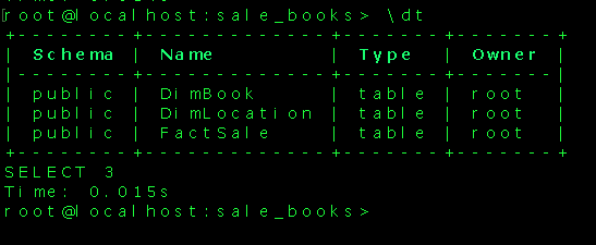
We have successfully created the tables in our DWH and we can now go ahead and populate the tables with data using another python script etl.py.

#importing necessary libraries
import pandas as pd
from sqlalchemy import create_engine
import psycopg2
import warnings
warnings.filterwarnings('ignore')
from clean_book import clean_book_genre

#reading from config file
config = {}
exec(open('config.py').read(), config)
user = config['user']
password = config['password']
port = config['port']
db = config['db']

# Connect to the PostgreSQL database server
engine = create_engine(f'postgresql://{user}:{password}@localhost/{db}')
conn = engine.connect()

# read transactional csv file as a dataframe
df_sales= pd.read_csv("book_sale.csv")
#read city-region from region.csv
region = pd.read_csv('region.csv')

The script can be run from the terminal/command prompt using the command python3 etl_dwh.py.

# creata a dataframe for book dimension table
book_id = 10000 # the book_id starts from this number 
df_book = df_sales[['book','genre']]
df_book.drop_duplicates(keep='first', inplace=True)
#in case book and genre is not matching for all rows call function to clean df_book
if (df_book.shape[0] != df_book['book'].nunique()):
    df_book = clean_book_genre(df_book)
df_book['bookid'] = pd.RangeIndex(book_id, book_id + len(df_book)) + 1
#load data into tables
df_book.to_sql(name="DimBook", con=conn, schema="public", if_exists="append", index=False)
print("Book Dimension Table data loading completed")

#create a dataframe for location dimension table
location_id = 50000
df_location = df_sales[['store']]
df_location.rename(columns = {'store':'city'}, inplace = True)
df_location.drop_duplicates(keep='first', inplace=True)
df_location['locationid'] = pd.RangeIndex(location_id, location_id + len(df_location)) + 1
df_location= pd.merge(df_location, region, on=['city'])
#load data into table
df_location.to_sql(name="DimLocation" ,con=conn,schema="public", if_exists='append',index=False)
print("Location  Dimension Table data loading completed")

#creata a fact table
fact_id = 0
df_fact = df_sales.copy()
df_fact.rename(columns = {'date':'dateid'}, inplace = True)
df_fact['rowid'] = pd.RangeIndex(fact_id, fact_id + len(df_fact)) + 1 # rowid for fact table
df_location.rename(columns = {'city':'store'}, inplace = True) # to match fact and dim table columns
df_fact= pd.merge(df_fact, df_location,how='left', on=['store']) # merge factsale and dimlocation tables
df_fact= pd.merge(df_fact, df_book,how='left', on=['book']) # merge factsale ad dimbook tables
df_fact = df_fact[['rowid','bookid','locationid','dateid','sale']] # filter factsale as per schema defineds
#load data into fact table
df_fact.to_sql(name="FactSale", con=conn, schema="public",if_exists='append',index=False)
print("Fact Table data loading completed")

#clean_book.py
import pandas as pd 
#function to clean book-genre 
# book-genre value should be unique pair in book dimension table
# we assume first instance book-genre pair as correct entry
def clean_book_genre(df_book):
    df_book_cleaned = pd.DataFrame(columns=['book','genre'])
    master_list_book =[]
    for index,row in df_book.iterrows():
        if row['book'] not in master_list_book:
            df_book_cleaned = df_book_cleaned.append(row, ignore_index = True)
            master_list_book.append(row['book'])
    return df_book_cleaned

 

That looks good! The fact and dimension tables have been populated with source data. The DWH is ready to run a query to get meaningful information. We can write a query to fetch the total number of each book sold citywide from the data(in descending order of total numbers sold).

SELECT L.city ,  b.book,SUM(s.sale) AS Total_No_Sold 
 FROM public."FactSale"  s
JOIN  public."DimBook" as b ON s.bookid = b.bookid
JOIN public."DimLocation" as L ON s.locationid = L.locationid
GROUP BY (L.city,b.book)  
ORDER BY SUM(s.sale) DESC
LIMIT 5;

The running of this query provides the following result

 

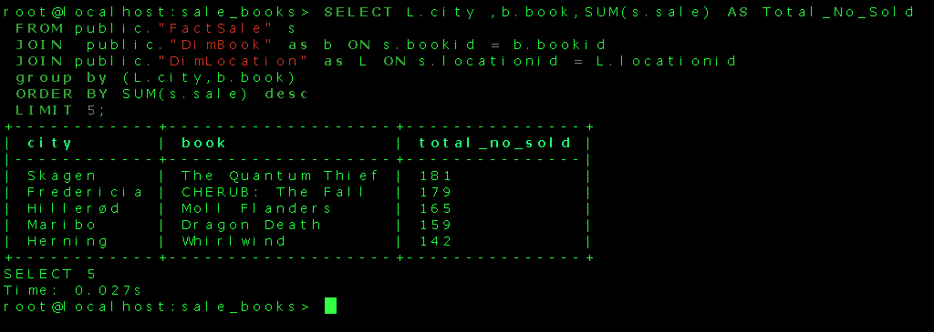
The simple DWH design can cater to fetch meaningful information from the data to aid business decisions. In large tables , the DWH could be optimized by techniques like partitioning and clustering. These optimization helps to improve query performance and facilitate easy management of data. The partition of data divides it into smaller manageable parts for easy retrieval of queries. The clustering aggregates rows of data based on similarity. The data in the DWH can be further processed and visual reports can be created using a tool like PowerBI.

Conclusion

The writeup explored a few of the aspects of a Data Warehouses through a hands-on exercise to design a simple star schema and an ETL pipeline to load data into the PostgreSQL database. The key takeaways from the study are as follows:

 The media shown in this article is not owned by Analytics Vidhya and is used at the Author’s discretion.

Subramanian Hariharan

A Marine Engineering professional with more than 29 years experience with a passion to leverage data for business solutions. I am a post graduate In Mechanical Engineering with experiences ranging from Operations, Production, Project Management, Quality Management and Data Analytics. I have also completed Advanced Certification in Data Science from Thayer School of Engineering , University of Dartmouth. I strongly believe learning is continuous process for growth in life and sharing knowledge builds a sense of community