Insurance Charges Prediction Using MLIB

This article was published as a part of the Data Science Blogathon.

Introduction on MLIB

In this MLIB  article, we will be working to predict the insurance charges that will be imposed on a customer who is willing to take the health insurance, and for predicting the same PySpark’s MLIB library is the driver to execute the whole process of this Machine learning pipeline.

We are gonna work with the real-world insurance dataset that I’ve downloaded from Kaggle. I’ll be providing the link for your reference, so without any further wait let’s get started.

Importing All the Libraries from PySpark

Our very first step is to import all the libraries from PySpark which will be required in a complete machine learning process i.e. from the data preprocessing to the model building phase.

from pyspark.sql import SparkSession
from pyspark.ml.stat import Correlation
import pyspark.sql.functions as func

Firstly we imported the SparkSession from PySpark to set up the spark session and then the Correlation library which eventually help in finding the colinearity between the two variables finally the last imported the functions module which will allow us to use predefined statistical functions of PySpark.

Setting Up the Spark Session for the PySpark MLIB Package

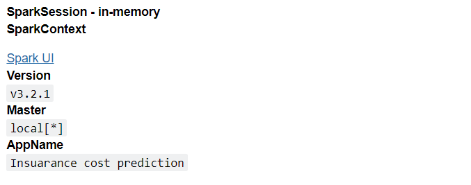
In this step, the Spark object will be created through which we can access all the deliverables, functions, and libraries that Spark has to offer. The new virtual environment will be created so that we can do all the steps involved in the ML pipeline.

spark  = SparkSession.builder.appName("Insuarance cost prediction").getOrCreate()
spark

Output

Reading Insurance Dataset Using Pyspark MLIB

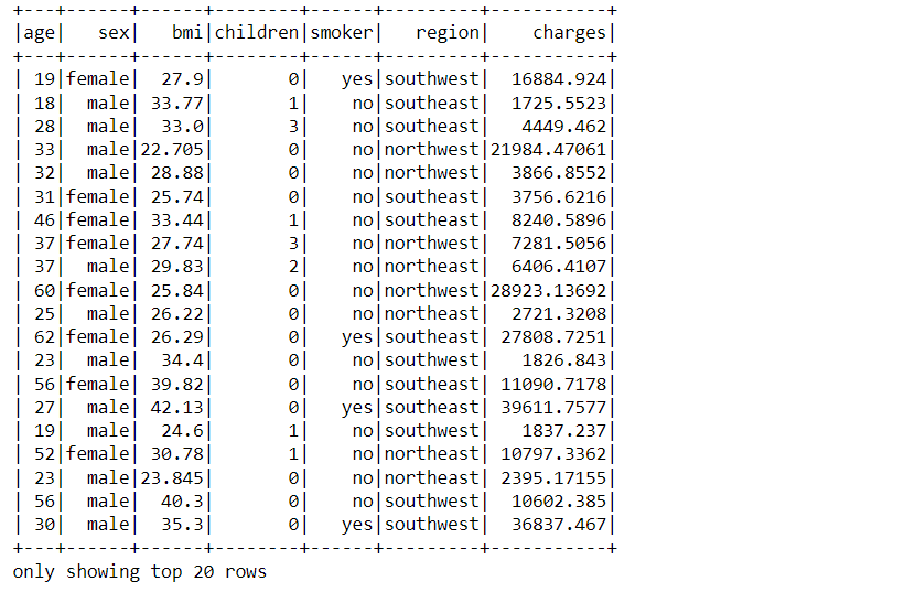
In this section, we will be reading the dataset using the read.csv() function of PySpark before moving forward with the further process let’s know more about the dataset.

So in this particular dataset, we have all the essential high-priority features that could help us to detect the life insurance charges which are possible to embrace on the card holders.

Features are as Follows

1. Age: Age of the customer.
2. BMI: Body Mass Index of the individual.
3. Children: Number of children he/she has.
4. Smoker: Is that individual a frequent Smoker or not.
5. Region: Which region/part he/she lives in and,

The charges column is our target/independent feature.

data = spark.read.csv("insurance.csv", inferSchema = True, header = True)
data.show()

Output:

Now it’s time to statistically analyze our dataset for that we will start by extracting the total number of records that are present in it.

data.count()

Output

1338

Inference: So from the above output we can state that there is a total of 1338 records in the dataset which we were able to get with the help of the count function.

print("Total number of columns are: {}".format(len(data.columns)))
print("And those columns are: {}".format(data.columns))

Output:

Total number of columns are: 7
And those columns are: ['age', 'sex', 'bmi', 'children', 'smoker', 'region', 'charges']

Inference: In the above code we tried to get as much information about the columns present for the analysis and conclusively we got to know that it has a total of 7 columns and their name as well.

Now let’s look at the Schema i.e. the structure of the dataset where we would be able to know about the type of each column.

data.printSchema()

Output

Inference: So from the above output we can see that adjacent to each feature we can see its data type and also a flag condition where it states whether the column can have null values or not.

Note: If you closely look at the result then one can see the sex, children, smoker, and region features are in the string format but they are categorical variables hence in the coming discussion we will convert them.

Now it’s time to see the statistical inferences of the dataset so that we can get some information related to the count, mean, standard deviation, and minimum and maximum values of the corresponding features.

data.describe().show()

Output

Inference: So from the above output we can draw multiple inferences where we can see each feature count is the same i.e. 1338 which means there are no Null values and the maximum age in the data is 64 while the minimum is 18 similarly max number of children are 5 and minimum is 0 i.e. no child. So we can put into the note that describes function can give ample information.

There is one more way to see the records and this one is similar to the ones who have previously come across pandas data processing i.e. head function.

data.head(5)

Output

Inference: As one can notice that it returns the row object so from here we can assume that if we want to analyze the data per record i.e. of each tuple then grabbing them using the head function could be a better approach.

Correlation in Variables

Correlation is one of a kind technique that helps us in getting more accurate predictions as it helps us know the relationship between two or more variables and return how likely they are positively or negatively related to it.

In this particular problem statement, we will be finding the correlation between all the dependent variables (continuous/integer one only) and the independent variables.

age = data.corr("age", "charges")
BMI = data.corr("bmi", "charges")

print("Correlation between Age of the person and charges is : {}".format(age))
print("Correlation between BMI of the person and charges is : {}".format(BMI))

Output

Correlation between Age of the person and charges is : 0.299008193330648
Correlation between BMI of the person and charges is : 0.19834096883362903

Inference: The correlation between the Age and insurance charges is equivalent to 0.30 while BMI and insurance charges are related to each other with a 0.20 value.

Note: We have only used two variables though logically we have multiple options they are in the string format so we can’t put them in this analysis, for now, you guys can repeat the same process for them after the conversion step.

String Indexer

In this section of the article, we will be converting the string type features to valid categorical variables so that our machine learning model should understand those features as we know that the ML model only works when we have all the dependent variables in the numerical format.

Hence, it is a very important step to proceed for this StringIndexer function will come to the rescue.

Note: First we will be converting all the required fields to categorical variables and then look at the line-by-line explanation.

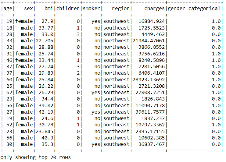
1. Changing the string type “sex” column to a categorical variable using String Indexer.

from pyspark.ml.feature import StringIndexer

category = StringIndexer(inputCol = "sex", outputCol = "gender_categorical")
categorised = category.fit(data).transform(data)

categorised.show()

Output

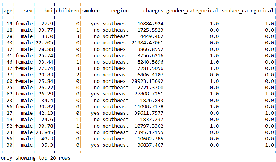
2. Changing the string type “smoker” column to a categorical variable using String Indexer

category = StringIndexer(inputCol = "smoker", outputCol = "smoker_categorical")
categorised = category.fit(categorised).transform(categorised) 

# Note that here I have used categorised in place of data as our updated data is in the new DataFrame i.e. "categorised"
categorised.show()

Output

3. Changing the string type “region” column to a categorical variable using String Indexer.

category = StringIndexer(inputCol = "region", outputCol = "region_categorical")
categorised = category.fit(categorised).transform(categorised)

categorised.show()

Output

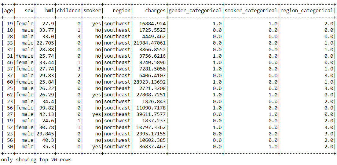
Code Breakdown

1. Firstly we imported the StringIndexer function from the ml. feature package of Pyspark.
2. Then for converting the sex column to a relevant categorical feature we took up the imported object and in the input parameter original feature was passed while in the output column feature we passed the name of the converted feature.
3. Similarly, we did the same for all the columns that were required to be converted to categorical variables.

Vector Assembler

As we already know that PySpark needs the combined level of features i.e. all the features should be piled up in a single column and they all will be treated as one single entity in the form of a list.

from pyspark.ml.linalg import Vector
from pyspark.ml.feature import VectorAssembler

Inference: So we have imported the Vector from the ML package and VectorAssembler from the feature package of ML so that we can pile up all the dependent fields.

categorised.columns

Output

['age',
 'sex',
 'bmi',
 'children',
 'smoker',
 'region',
 'charges',
 'gender_categorical',
 'smoker_categorical',
 'region_categorical']

Inference: The columns which one can see in the above output are the total columns but we don’t need the string ones instead the ones which were changed to the integer type.

concatenating  = VectorAssembler(inputCols=["age","bmi", "children", "gender_categorical", "smoker_categorical", "region_categorical"],
                                 outputCol="features")
results = concatenating.transform(categorised)

Inference: While combining all the features we pass in all the relevant column names in the form of a list as the input column parameter and then to see the changes as well we need to transform our original dataset as well.

for_model = results.select("features", "charges")
for_model.show(truncate=False)

Output

 

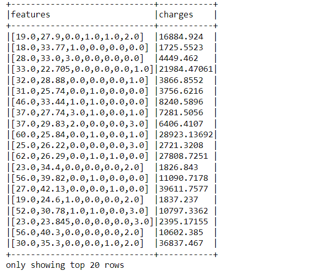
Inference: Now we are creating a new DataFrame which we will send it across to our model for model creation.

Note: In the show function we have used truncate=False which means now all the features in the list will show up.

Train Test Split on MLIB

So by far, we have done each step that is required in the model building phase hence now it’s time to split out the dataset into training and testing forms so that one will be used for training the model and the other one will be to test the same.

train_data, test_data = for_model.randomSplit([0.7,0.3])

Inference: In the above random split() function we can see that the training data is 70% (0.7) and the testing data is 30% (0.3).

train_data.describe().show()

Output

test_data.describe().show()

Output:

 

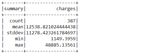
Inference: Describe function is used on top of both the split dataset and we can see multiple information about them like the total count of the training set is 951 while the other one has 387.

Model Building

In this phase of the article, we will be building our model using the Linear Regression algorithm as we are dealing with a continuous group of features so this is the best and go-to choice for us in the current possible problem statement.

from pyspark.ml.regression import LinearRegression

lr_model = LinearRegression(featuresCol= "features",
                            labelCol="charges")
lr_model

Output

Firstly we are embedding a Linear Regression object by passing in the features column that we have already separated and the label column is our target feature i.e. “charges“.

training_model = lr_model.fit(train_data)
training_model

Output

LinearRegressionModel: uid=LinearRegression_d7bb227324ac, numFeatures=6

Then the LR object which we have created fits with the training data that we got from the random split() method, in the output one can see it returned the valid information about the model i.e. the number of features it holds – 6.

Model Evaluation on MLIB

So by far, we are now done with the model development phase so it’s time to evaluate the model and get the inference of the same about whether it is a worthy model or not.

output = training_model.evaluate(train_data)

Evaluate function is to call all the metrics that are involved in the model evaluation phase so that we can decide the accuracy of the model.

print(output.r2)
print(output.meanSquaredError)
print(output.meanAbsoluteError)

Output

0.7477904623279588
38900867.48971935
4324.864277057295

Here are the results of all the valid evaluation metrics available:

1. R-squared: This metric explains how much variance of the data is explained by the model.
2. Mean Squared Error: This returns the residual values of a regression fit line and magnifies the large errors
3. Mean Absolute Error: Does the same thing but this one focuses on minimizing the small errors which MSE might ignore.

It’s time to make predictions!!

features_unlabelled_data = test_data.select("features")
final_pred = training_model.transform(features_unlabelled_data)
final_pred.show()

Output

 

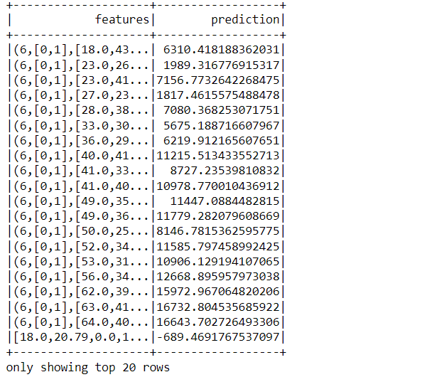
Code breakdown: This is the final step where we will be doing the predictions based on the model we have built and comparing the actual result with the predicted one.

1. Created a DataFrame for the unlabelled data i.e. our features column
2. Then we transformed the unlabelled data using the same function we used before.
3. At the last, we show the prediction results which one can see in the above output.

Conclusion on MLIB

Finally, we can predict the insurance charges with the help of Pyspark’s MLIB library we have performed every step from the ground level i.e. from reading the dataset to making the predictions from the evaluated model.

Let’s discuss in a descriptive way whatever we have learned so far!

1. First of all, we read the insurance dataset which was a real-world dataset from Kaggle
2. Then we performed the data preprocessing steps where we got to know about the dataset’s columns, statistics, and changing the string type columns to categorical variables.
3. Then comes the Model building phase where we build the Linear Regression model using Pyspark’s MLIB library.
4. At the last, we evaluated the model and made the predictions from the same.

 The media shown in this article is not owned by Analytics Vidhya and is used at the Author’s discretion.

Aman Preet